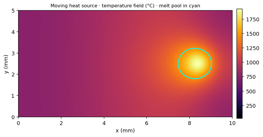
How to model a melt pool
This is the moving heat source in welding and 3D-printed metal. A melt pool moves and leaves a tail of heat. We solve it on the transient field engine of physicsbase. We check it against the classic Rosenthal solution.
Read the post →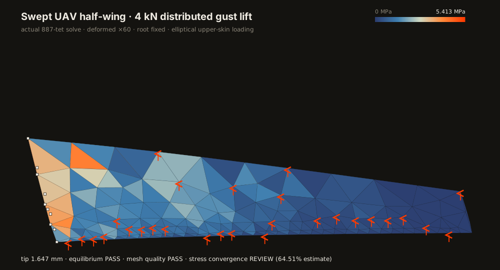
One CAD path, five kinds of physics
Animated XYZ wind vectors, temperature, diffusion, rigid-stop contact and damage screening on pinned STEP models—without flattening the result.
A gust load should touch the wing, not just its tip
We generate a swept UAV wing STEP, map an elliptical lift law onto its upper surface, run the real tetrahedral solve, and publish the load-discretization check.
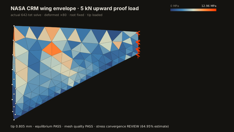
From a NASA wing STEP to a live proof-load solve
We pin an official NASA Common Research Model wing, derive a transparent live-size solid, run a 5 kN load, and publish both the result and its mesh-convergence warning.
quasi-isotropic
Ex = (U1²−U4²)/U1
Three composite benchmarks, from the papers
The Tsai-Pagano invariants, the Tsai-Wu failure criterion, and the WWFE reference lamina. The laminate engine reproduces them to machine precision.
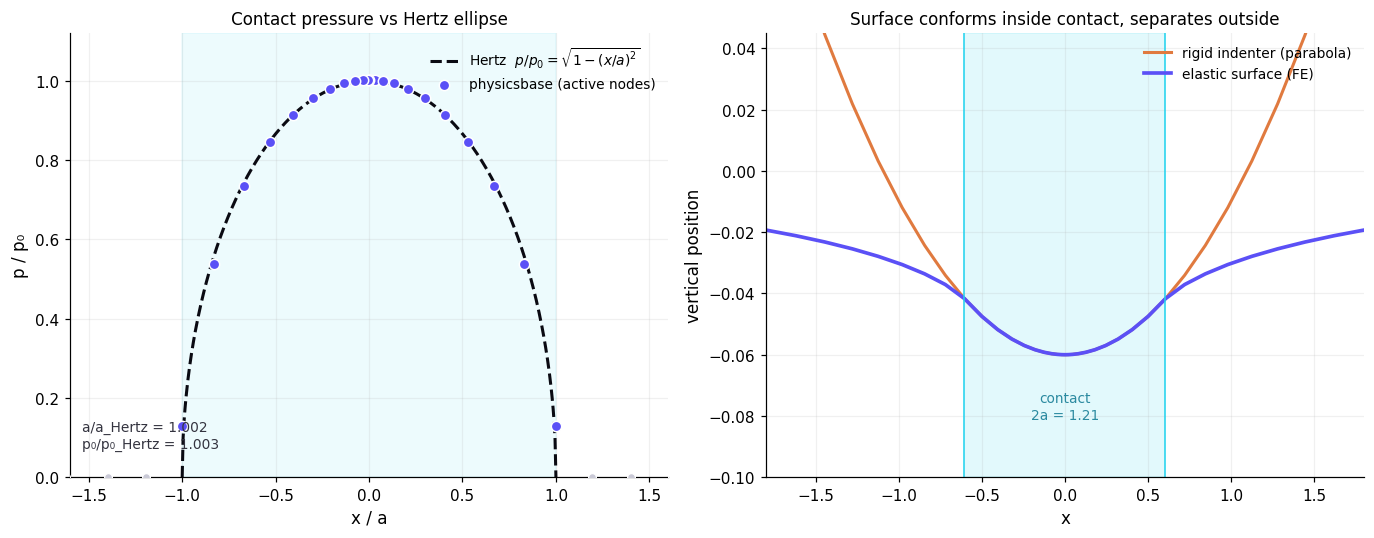
The first problem in contact mechanics
A rigid cylinder presses into an elastic half-space. We solve it with an exact active-set contact method. There is no penalty parameter. The result agrees with the 1882 Hertz pressure ellipse to 0.3%.
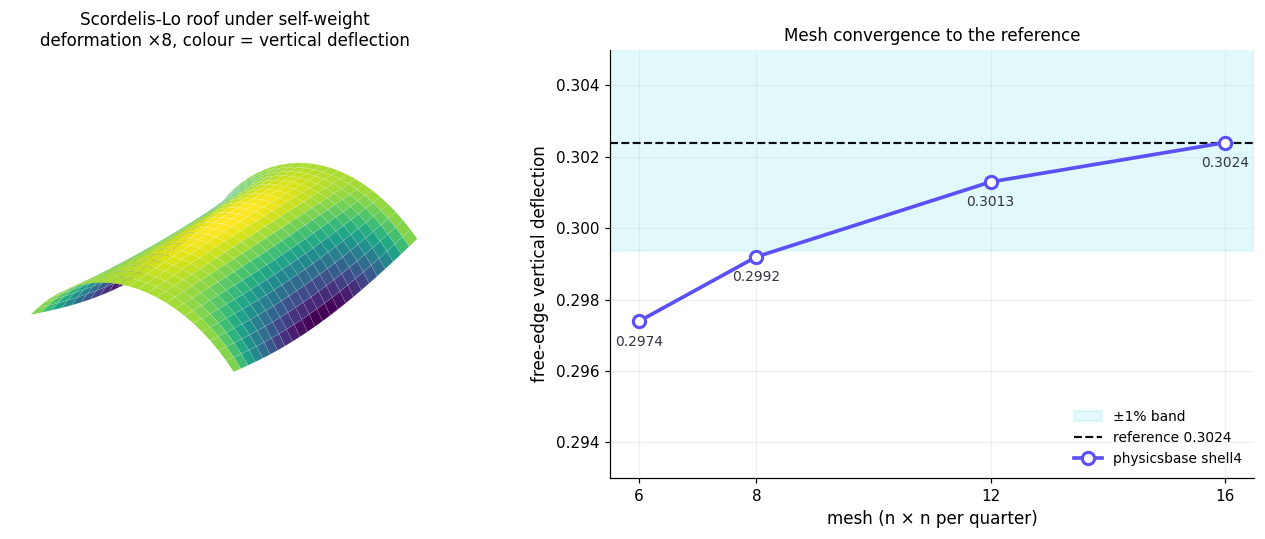
How the shell4 element passes its benchmark
A flat-facet shell4 element. The drilling-DOF trap makes it 40% too soft. One term corrects it. The result passes the Scordelis-Lo roof to 1% of the MacNeal and Harder reference.
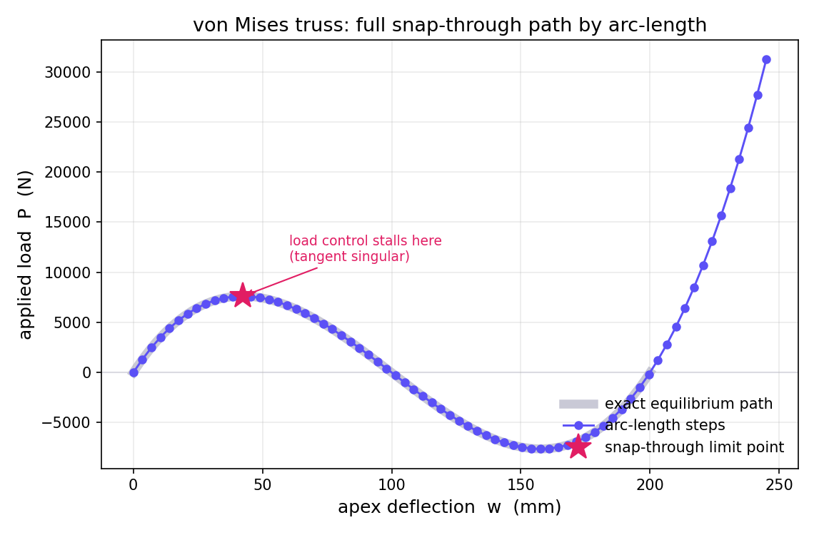
How to solve past a limit point
Geometric nonlinearity and the Crisfield arc-length method follow the full von Mises snap-through path. This path goes through the limit point that load control cannot cross. The result matches the exact curve to 1e-15.
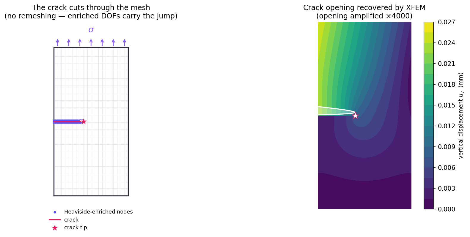
A crack inside the mesh
The eXtended Finite Element Method on physicsbase. A crack cuts through the elements. There is no new mesh. We get K₁ from the energy release rate. It is within 1.5% of the handbook.
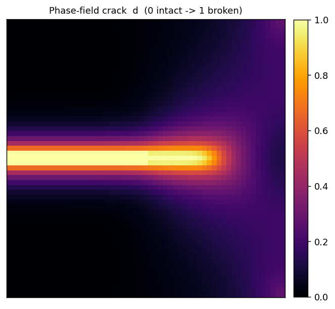
How a crack grows on its own
Two physics in a loop. This is the single-edge-notched fracture benchmark. It couples the structural and field solvers of physicsbase. The crack grows on its own.
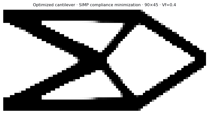
How the structure designs itself
The classic SIMP topology-optimization method on the engine. An optimization loop contains an FE solve. This gives the well-known optimized cantilever. The full code is included.
One kernel, many physics
How one scalar-field solver does heat conduction, mass diffusion, potential flow, and transport. They are all the same equation with different labels.
How we numerically verify a physics engine
The system checks recorded implementation claims against analytical and discrete references. This is a tour of the verification suite—and the limits it cannot cross.