A crack inside the mesh.
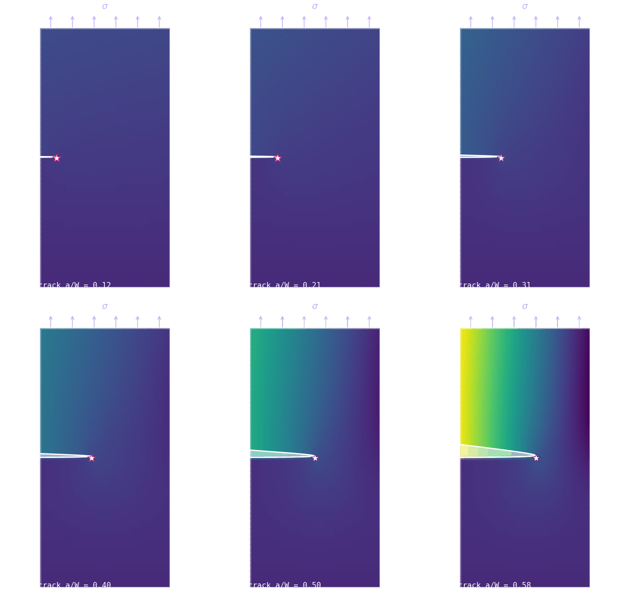
Ordinary finite elements cannot represent a crack unless you cut the mesh to fit it. Thus you make a new mesh each time the crack moves. The eXtended Finite Element Method removes that rule. The crack runs through the elements. A few extra unknowns let the displacement jump across it. We built it on physicsbase. We got the textbook stress-intensity factor to within 1.5%.
A crack is a tear in the displacement field. On one side the material moves up. On the other side it stays. At the crack face the two sides are not connected. Finite elements use the opposite assumption. Inside each element the displacement is a smooth polynomial that interpolates the corner nodes. These two facts give the oldest problem in computational fracture. To model a crack with plain elements, the crack must run along element edges. You must rebuild the mesh to follow the crack as it grows. For decades, fracture codes were, in effect, advanced re-meshers.
Belytschko and Black, and Moës, Dolbow, and Belytschko, introduced the eXtended Finite Element Method (XFEM) in 1999. It made re-meshing optional. Keep a simple, structured mesh. Let the crack cut through the middle of elements anywhere. Then, for the elements that the crack passes through, add extra degrees of freedom. Their job is to carry the jump. The mesh does not need to know where the crack is. The enrichment knows. This article is about how we add that capability to physicsbase. As in the other articles, it is about where the engine ends and the new physics begins.
The one equation that does the trick
Standard FEM writes the displacement in an element as a sum over its nodes: \( \mathbf{u}^h(\mathbf{x}) = \sum_i N_i(\mathbf{x})\,\mathbf{u}_i \). The \(N_i\) are the usual shape functions. XFEM keeps that term and adds a second term:
\[ \mathbf{u}^h(\mathbf{x}) = \underbrace{\sum_{i} N_i(\mathbf{x})\,\mathbf{u}_i}_{\text{ordinary FE}} \;+\; \underbrace{\sum_{j\in\mathcal{E}} N_j(\mathbf{x})\,\big(H(\mathbf{x}) - H(\mathbf{x}_j)\big)\,\mathbf{a}_j}_{\text{crack enrichment}} \]
The new unknowns \(\mathbf{a}_j\) are only on the nodes \(\mathcal{E}\) of the elements that the crack cuts. The multiplier \(H(\mathbf{x})\) is the Heaviside sign function. It is \(+1\) on one side of the crack and \(-1\) on the other. It changes sign across the crack face. Thus the enriched term can represent a clean discontinuity inside an element, with no element edge. The shift \(-H(\mathbf{x}_j)\) is a bookkeeping step. It makes the enrichment zero at the nodes. Thus the ordinary \(\mathbf{u}_i\) still equal the nodal displacements, and the boundary conditions stay simple.
What physicsbase supplies, and what XFEM adds
The benchmark is the single-edge-notch tension specimen (SENT). It is a rectangular plate with a horizontal crack cut in from the left edge to a depth a. It is pulled in uniform tension \(\sigma\). It is the first example in fracture. It has a handbook answer to check against.
The engine gives the physics of a plain elastic quad: the constitutive law and the strain-displacement operator. We build everything the crack needs from those. The request and response boundary is small and clear:
from femengine.materials import Material

D = Material(E=210e9, nu=0.3).plane_strain_D()   # (3,3) stress = D · strain

# out: the same 3×3 the engine uses for any plane-strain stress analysis
# [[ 2.83e11  1.21e11  0      ]
#  [ 1.21e11  2.83e11  0      ]
#  [ 0        0        8.08e10 ]]
From there the XFEM layer builds each element stiffness \( \mathbf{k}_e = \int_{\Omega_e} \mathbf{B}^\top \mathbf{D}\, \mathbf{B}\,\mathrm{d}\Omega \) in the usual way. But the strain-displacement matrix \(\mathbf{B}\) gets extra columns for the enriched nodes. Those columns are the ordinary shape-function derivatives multiplied by the shifted sign function:
# standard columns (every node): the usual quad B-operator
B[0, 2*i]   = dNdx[i]
B[1, 2*i+1] = dNdy[i]
B[2, 2*i]   = dNdy[i];  B[2, 2*i+1] = dNdx[i]

# enriched columns (cut-element nodes only): same derivatives × jump
psi = Hs - H_node          # shifted Heaviside: H on this sub-cell minus H at the node
B[0, col]   = dNdx[i] * psi
B[1, col+1] = dNdy[i] * psi
B[2, col]   = dNdy[i] * psi;  B[2, col+1] = dNdx[i] * psi
There is one detail that the engine cannot handle for us. It is the key part of XFEM integration. The integrand \( \mathbf{B}^\top\mathbf{D}\,\mathbf{B} \) is now discontinuous inside a cut element. Ordinary Gauss quadrature assumes a smooth integrand. Thus it would get the area of each side of the crack wrong. So we split every cut element into two sub-cells: one above the crack and one below. We integrate each one separately. We hold \(H\) to its constant value (\(+1\) or \(-1\)) on that side:
for Hs, lo, hi in ((+1.0, 0.0, 1.0), (-1.0, -1.0, 0.0)):   # top half, bottom half
    for gx, gy in gauss_2x2:
        B = Bmat(node_coords, enriched, gx, remap(gy, lo, hi), Hs)
        ke += B.T @ D @ B * detJ * sub_scale        # D straight from physicsbase
Getting K₁ without touching the crack tip
Engineers do not want the displacement field for its own sake. They want the stress-intensity factor \(K_I\). This one number says how hard the crack tip is opened and whether the part will fail. The textbook method to get it from a simulation is a special contour integral around the tip. That method needs extra "branch-function" enrichment there. We took the simpler route on purpose: the energy release rate.
Griffith showed that a crack advances when the structure can release stored elastic energy as it grows. The energy released per unit of new crack area is \(G = \mathrm{d}U/\mathrm{d}a\). For a linear-elastic material it links directly to the stress-intensity factor:
\[ G = \frac{\mathrm{d}U}{\mathrm{d}a}, \qquad K_I = \sqrt{E'\,G}, \qquad E' = \frac{E}{1-\nu^2}\ \text{(plane strain)} \]
This fits an engine well, because \(U = \tfrac12\,\mathbf{u}^\top \mathbf{K}\,\mathbf{u}\) is the strain energy of a solved model. physicsbase already computes it. We solve the specimen at two crack lengths, one element shorter and one longer. Then we take a central difference:
def stress_intensity(W, L, nx, ny, material, a, sigma):
    da = W / nx
    for aa in (a - da, a + da):              # crack one element shorter / longer
        m = XFEMCrack(W, L, nx, ny, material, aa)
        _, U[aa] = m.solve(sigma)            # strain energy of the solved model
    G  = (U[a+da] - U[a-da]) / (2*da)      # energy release rate  dU/da
    return np.sqrt(Eprime(material) * G)     # K_I = sqrt(E' G)
There is no tip enrichment, no interaction integral, and no fragile near-tip stress sampling. There are only two solves and a finite difference. Energy is a global quantity. Thus it is more forgiving than a reading of the singular stress field at the tip. This is why this route stays accurate with plain Heaviside enrichment.
What came out
We ran a plate of width \(W=1\) and height \(2W\), with Young's modulus 210 GPa and \(\nu=0.3\), under unit remote tension. The crack cuts through the middle row of elements. The enriched nodes and the recovered opening look like this:
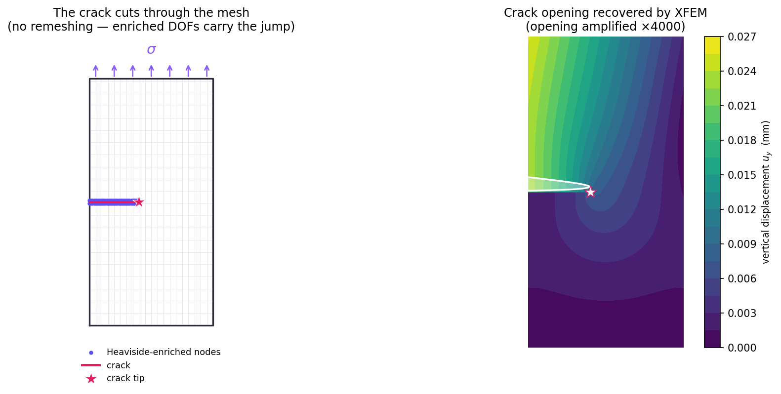
The important number is \(K_I\). The handbook value for this geometry is \(K_I = \sigma\sqrt{\pi a}\,F(a/W)\), with the standard edge-crack polynomial \(F(\alpha) = 1.12 - 0.231\alpha + 10.55\alpha^2 - 21.72\alpha^3 + 30.39\alpha^4\). We compared across three crack depths and two mesh densities:
| Crack depth a/W | Mesh | K₁ — XFEM | K₁ — handbook | Error |
|---|---|---|---|---|
| 0.30 | 40 × 41 | 1.5545 | 1.6115 | −3.54% |
| 0.40 | 40 × 41 | 2.2811 | 2.3580 | −3.26% |
| 0.50 | 40 × 41 | 3.3993 | 3.5423 | −4.04% |
| 0.30 | 80 × 81 | 1.5819 | 1.6115 | −1.83% |
| 0.40 | 80 × 81 | 2.3225 | 2.3580 | −1.50% |
| 0.50 | 80 × 81 | 3.4672 | 3.5423 | −2.12% |
Notice two things. First, the answers are close to the handbook across the whole range of crack depths, within a few percent, from a method that never meshed the crack. Second, and more important, the error halves when the mesh gets finer: from about 3.5% at 40×41 to about 1.5% at 80×81. This is the sign of a convergent method. The discretisation error goes toward zero. It does not stay at a fixed modelling bias. The remaining gap is the cost of plain Heaviside enrichment without the extra crack-tip branch functions. It keeps closing as the mesh gets finer.
Why this one is a good stress test
Topology optimization was one physics in a loop. Phase-field fracture was two physics in a loop. XFEM is different again. Here the approximation space itself changes. The unknowns are no longer only "displacement at nodes." Some are jump amplitudes with a sign function. The quadrature must respect a discontinuity that ignores element boundaries. physicsbase gives the constitutive matrix and shape-function derivatives, so enrichment can be added on top. The part that is "just an elastic quad" remains numerically verified code; the XFEM-specific evidence must still be assessed separately.
Honest footnotes
We used Heaviside (jump) enrichment only. We placed the crack tip on an element boundary, so the tip is in a single column of nodes. Thus we could skip the near-tip branch-function enrichment that a production XFEM code adds. We get \(K_I\) from the global energy release rate. We finite-difference the strain energy in the crack length. We do not use an interaction (M-) integral. The energy route is robust and mesh-convergent. But it does not separate mixed-mode \(K_I\) and \(K_{II}\). Here the loading is pure mode I by symmetry. The formulation is standard and common to the references below. The code is our own. It reuses none of the published implementations. The point, as in the other case studies, is narrow. A general-purpose FE engine, given only its own constitutive matrix and shape functions, reproduces a fracture-mechanics benchmark to within a percent or two. It also converges as you refine the mesh.
References
- T. Belytschko & T. Black, "Elastic crack growth in finite elements with minimal remeshing," Int. J. Numer. Methods Eng. 45 (1999), 601–620.
- N. Moës, J. Dolbow & T. Belytschko, "A finite element method for crack growth without remeshing," Int. J. Numer. Methods Eng. 46 (1999), 131–150.
- D. Datta, "Introduction to eXtended Finite Element (XFEM) Method" (2013). arXiv:1308.5208
- A. R. Jimenez et al., "An eXtended Finite Element Method Implementation in COMSOL Multiphysics: Solid Mechanics" (2021). arXiv:2109.03153
- H. Tada, P. C. Paris & G. R. Irwin, The Stress Analysis of Cracks Handbook, 3rd ed. (ASME Press, 2000) — edge-crack geometry factor.
examples/xfem.py. It has a Heaviside-enriched Quad4, sub-cell integration, and the energy-release-rate K₁, on top of physicsbase's Material. Read the docs →