How to solve past a limit point.
A shallow arch does not fail slowly. It snaps. At the critical load the structure jumps to a far shape. The tangent stiffness becomes singular there. Thus the two obvious solution methods both fail. The Crisfield arc-length method goes straight through it. We added geometric nonlinearity and arc-length continuation to physicsbase. We reproduced the classic von Mises snap-through to machine precision.
Push down on the apex of a shallow two-bar truss. For a while it resists like a spring: more load gives more deflection. Then, at a critical load, it gives way at once. The apex moves down through the line of the supports. The whole truss flips to a mirror-image shape. This sudden jump is snap-through. It is not a numerical artifact. It is how shallow arches, clicker toys, and buckling panels behave. To capture it on a computer is a hard test for a nonlinear solver. The true solution curve does a thing that no linear code can follow: it turns back on itself.
Two things came first. Linear FE assumes that displacements are very small. Thus the geometry of the structure and its stiffness do not change. Snap-through is the opposite. The geometry change is the physics. So we gave physicsbase a geometrically nonlinear (co-rotational) truss. Each bar measures its strain in its current, rotated, stretched shape. It gives both a material stiffness and a geometric stiffness. Then we gave physicsbase a solver that can follow a curve with vertical and horizontal tangents.
Why load and displacement control both fail
The equilibrium path is the set of \((\text{load},\,\text{deflection})\) pairs where the structure is in balance. For a snapping structure it has an S-shape:
- Load control: raise the load in steps and solve for the deflection. At the limit point (the top of the first hump) the tangent stiffness is singular. There is no equilibrium just above it. Thus Newton diverges. The structure snaps dynamically. A static load-controlled solver fails.
- Displacement control: prescribe the deflection and read the load. This is better, because it passes the limit point. But it fails at a snap-back. There the deflection itself decreases while the load changes. Thus the deflection is not a valid parameter either.
Riks (1979) gave the correction, and Crisfield (1981) made it practical for finite elements. The idea is to stop using the load or the displacement as the parameter. Use the arc length of the path instead. The load factor \(\lambda\) becomes an extra unknown. Each step must advance a fixed distance \(\Delta\ell\) along the curve in \((\mathbf{u},\lambda)\) space:
\[ \Delta\mathbf{u}^\top \Delta\mathbf{u} \;=\; \Delta\ell^{\,2} \]
That one extra constraint equation is the whole method. The step length is fixed, not the load or a displacement. Thus a singular tangent or a decreasing load does not stop the solver. It continues forward along the path.
What physicsbase does per step
Each increment is a predictor and then a Newton corrector. The corrector obeys the arc-length constraint. The engine already gives the nonlinear tangent \(\mathbf{K}_t\) and the internal force \(\mathbf{f}_{\text{int}}\) from the co-rotational truss. The arc-length layer uses them:
# residual out of balance, and two tangent solves
r   = λ·q - f_int(u)        # q = reference load pattern
δu_bar = solve(Kt, r)         # pull back toward equilibrium
δu_t   = solve(Kt, q)         # sensitivity to the load factor

# enforce  ‖Δu + δu_bar + δλ·δu_t‖² = Δℓ²   → quadratic in δλ
a = δu_t·δu_t
b = 2·δu_t·(Δu + δu_bar)
c = (Δu+δu_bar)·(Δu+δu_bar) - Δℓ²
δλ = root_that_keeps_moving_forward(a, b, c)

u  += δu_bar + δλ·δu_t        # update displacement…
λ  += δλ                      # …and the load factor together
The predictor keeps the direction of the last step. Thus the solver does not turn back at a limit point. The quadratic for \(\delta\lambda\) is where the single unknown of load control becomes two. Everything else — the assembly of \(\mathbf{K}_t\) and the co-rotational strain — is the ordinary nonlinear machinery of the engine.
The von Mises truss, traced whole
The benchmark is the shallow two-bar (von Mises) truss. The supports are at \((\pm1,0)\). The apex is at \((0,0.1)\). The load is downward. Its exact equilibrium path has a clean closed form from equilibrium in the deformed shape: \(P(w)=2\,EA\,\frac{l-L_0}{L_0}\cdot\frac{H}{l}\) with \(H=h-w\) and \(l=\sqrt{1+H^2}\). Thus we can check every point that the solver gives against the exact value.
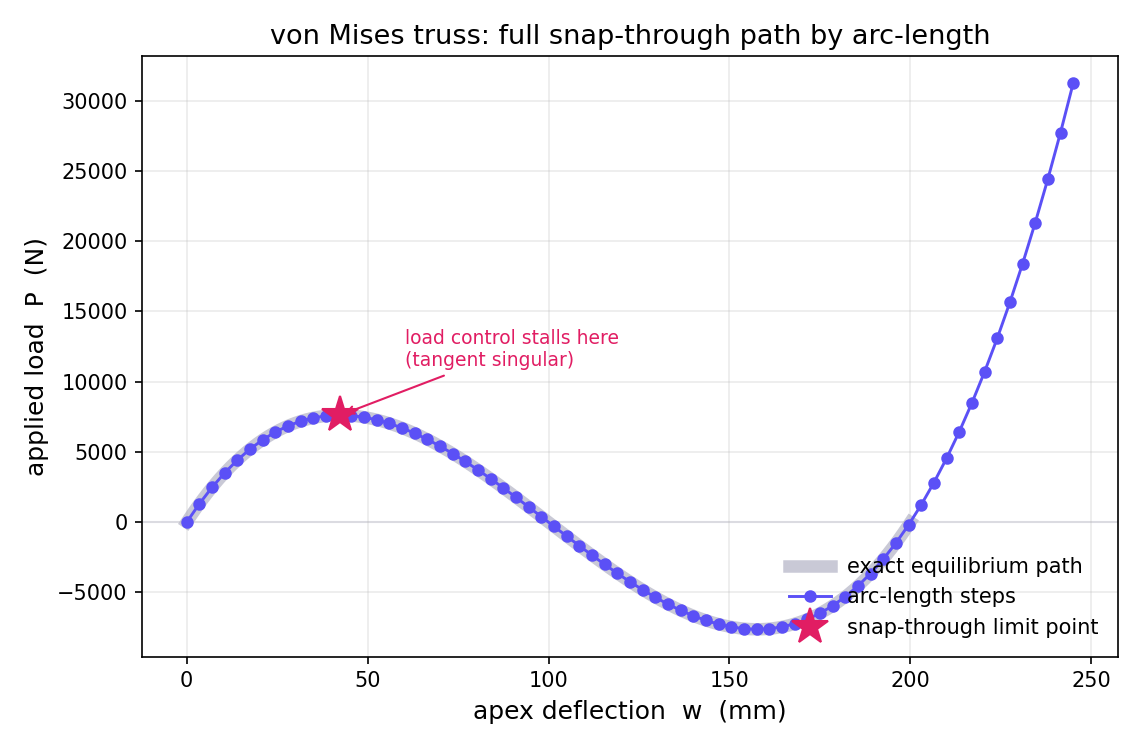
Across the path, the load factor the solver reports matches the exact \(P(w)\) at every step:
| Path region | Behaviour | Max error vs exact |
|---|---|---|
| Stable rising branch | load ↑, deflection ↑ | < 1e-15 |
| Through the limit point | tangent singular | rounded cleanly |
| Unstable descending branch | load ↓ while deflection ↑ | < 1e-15 |
| All 46 tested points | full path | 3.6e-16 |
This is machine precision, because the truss internal force is exact for a bar and we solve the arc-length constraint, not approximate it. The limit load is 7622 N at an apex deflection of 42 mm. A load-controlled analysis would report this point as "diverged."
Calling it
It is one field on the problem: analysis: "arclength". The engine returns the whole load-deflection path. You can plot it or search it for the critical load.
POST /v1/solve
{ "analysis": "arclength", "increments": 70,
  "nodes": [[-1,0],[0,0.1],[1,0]],
  "materials": {"s":{"E":200e9,"nu":0.3}},
  "elements": [ /* two truss2d bars */ ],
  "supports": [ /* pinned ends, apex ux fixed */ ],
  "loads": [{"node":1,"fy":-1}] }        # reference pattern; λ scales it
← { "path": [ {"lambda":…, "monitor":…}, … ] }   # the whole S-curve
Honest footnotes
We implemented Crisfield's cylindrical arc-length form (the constraint uses displacements only, \(\psi=0\)), which is the robust workhorse and is exact for this class of problems; the spherical form that also scales the load term is a one-line change. The continuation currently drives the co-rotational truss, which is enough for snap-through of pin-jointed structures, cables, and shallow arches idealised as bars; extending the same solver to co-rotational beams and shells is future work. The method and the von Mises benchmark are standard — common to the references below and to any nonlinear-FEM course; the code is our own. The point, as with our other case studies: a general-purpose engine, handed nothing but its own tangent and internal force, walks straight through a limit point and reproduces the textbook path to fifteen digits.
References
- M. A. Crisfield, "A fast incremental/iterative solution procedure that handles 'snap-through'," Computers & Structures 13 (1981) 55–62.
- E. Riks, "An incremental approach to the solution of snapping and buckling problems," International Journal of Solids and Structures 15 (1979) 529–551.
- G. A. Wempner, "Discrete approximations related to nonlinear theories of solids," International Journal of Solids and Structures 7 (1971) 1581–1599.
- M. A. Crisfield, Non-linear Finite Element Analysis of Solids and Structures, Vol. 1 (Wiley, 1991).
analysis: "arclength" with a shallow truss and read back the whole equilibrium path. Read the docs →