How a crack grows on its own.
It is hard to make a material break on a computer. Cracks are discontinuities, and finite elements do not handle discontinuities well. The phase-field method avoids this. It turns the crack into a smooth field. We reproduced the benchmark on physicsbase. It needed two engines that pass data to each other.
A structural engineer can usually point to where a part will fail. But it is one of the hardest problems in computational mechanics to make a computer show the crack form and grow. A crack is a moving discontinuity in the displacement field. Classic finite elements assume that the field is smooth. Thus, for decades, cracking meant a new mesh around the tip at each step, or special crack functions in the elements. Then a clever idea came. Do not track the crack as a surface. Represent it as a smooth phase field d. It goes from 0 (intact) to 1 (fully broken) over a thin band. A PDE decides where it grows. This is the phase-field method. It is now the main way to simulate brittle fracture.
It is also a good demonstration for physicsbase, because it is not one physics. It is two coupled physics. The displacement field needs a structural solve. The crack field needs a field solve. They pass results back and forth until they agree. Thus this article is about the boundary: what each solver sends the other.
The two fields, and how they talk
The benchmark is the single-edge-notched tension test (Bourdin et al. 2000; Miehe et al. 2010). It is a unit square with a horizontal pre-notch cut halfway in. It is clamped at the bottom. It is pulled straight up at the top. Two unknowns are on the same mesh:
- Displacement
u: a structural problem. Cracked material carries no load. Thus \(g(d) = (1-d)^2\) scales the stiffness of each element. Where the crack field is high, the element becomes soft. - Crack
d: a field problem. It solves a screened-Poisson equation. The stored elastic energy of the material drives it. Highly-strained material tends to crack.
You cannot solve either one alone. The stiffness depends on d. And d depends on the strain from u. Thus the solver alternates (a "staggered" scheme). The important thing is what passes between them each step.
Exchange 1 — the structural solve
The crack solver gives the structural solver a degraded structure: the same mesh, but the current damage reduces the effective stiffness of each element. physicsbase solves for the displacement. It reports the strain energy in each element. This energy feeds the crack.
# in:  the current design + how hard the top is pulled
elements: quad4 mesh, each stiffness scaled by  g = (1 - d)**2
supports: bottom edge clamped;  top edge  uy = Δ  (this load step)

# out: physicsbase returns the deformation and per-element stress
displacements: [ {"ux":…, "uy":…}, … ]
elements:      [ {"stress":[sxx,syy,txy], "strain":[…]}, … ]
reaction (top): 0.699          # the force the specimen is carrying
Exchange 2 — the crack solve
From those stresses the driver computes a crack-driving energy H for each element. It keeps H monotonic, so cracks never heal. It gives that field to the field solver. physicsbase returns the updated crack field, which is the shape of the damage.
# in:  a screened-Poisson PDE assembled from physicsbase field operators
#   ( Gc·l ∇²  +  (Gc/l + 2H) )  d  =  2H
conductivity: Gc·l        # crack surface energy × length scale
reaction:     Gc/l + 2H   # H = the driving energy from Exchange 1
source:       2H

# out: physicsbase returns the crack field, clamped irreversible
d: [ 0.02, 0.05, …, 1.00, 1.00, … ]   # 0 intact → 1 broken
Using physicsbase: two kernels, four operators
As coupled PDEs this looks like a research code. As physicsbase calls, the whole physics is a few operator evaluations: two from the structural element and three from the field element. Here is every piece that the engine gives. Everything else is glue code.
The elasticity side — from Quad4
Two calls. The first is the element stiffness, which the crack degrades for each element. The second is the strain-displacement operator of the element. We use it to read the elastic energy that drives cracking from the displacement solution:
from femengine.elements import Quad4
from femengine.materials import Material

sq = [[0,0],[h,0],[h,h],[0,h]]                          # one h×h cell
KE = Quad4.stiffness(sq, Material(E, nu), {"kind":"plane_strain"})  # (8,8)
B, _ = Quad4._B_at(sq, 0.0, 0.0)                          # (3,8) strain-disp at centre
D  = Material(E, nu).plane_strain_D()                      # (3,3) constitutive

# per element, from the solved displacements u_e:
eps = B @ u_e                 # strain  [εxx, εyy, γxy]
psi = 0.5 * eps @ (D @ eps)     # elastic energy density -> crack driving force
Nothing here is special. KE, B, and D are the same objects that the engine uses for an ordinary stress analysis. We scale KE by \(g(d) = (1-d)^2\) before assembly. We read the energy from the returned strain.
The crack side — from FieldQuad4
The phase-field equation \[ \big(G_c\, l\, \nabla^2 - (G_c/l + 2H)\big)\, d = -2H \] is a screened-Poisson problem. The physicsbase field element gives the three standard operators that build it. These are the same operators that build a heat-conduction problem:
from femengine.field.elements import FieldQuad4

Kc = FieldQuad4.conductivity(sq, 1.0, {})   # (4,4)  ∫∇N·∇N   — the diffusion term
Mc = FieldQuad4.capacitance(sq, 1.0, {})    # (4,4)  ∫N·N     — the reaction term
Fc = FieldQuad4.source(sq, 1.0, {})         # (4,)   ∫N       — the forcing term

# assemble the crack system element by element:
#   A = Gc·l · Kc   +   (Gc/l + 2H) · Mc            (H = driving energy per element)
#   b = 2H · Fc
# solve A d = b, then clamp d to [d_prev, 1]  (cracks never heal)
That is the whole "field" side. conductivity gives the crack its surface-energy smoothing. capacitance gives the reaction coefficient that adds the driving energy H. source is the forcing. These are three matrix templates from the same engine that solves temperature fields. We reuse them without change to grow a crack.
The loop that couples them
for step in load_steps:                # ratchet the top displacement up
    for _ in range(2):                   # staggered iterations
        u = solve_elasticity(KE, g(d))   # ← Quad4, degraded by the crack
        H = np.maximum(H, psi(u))         # energy from the solve, kept monotonic
        d = solve_phase(Kc, Mc, Fc, H)   # ← FieldQuad4, driven by the energy
for loop. The engine never learns what "fracture" means. It only returns stiffness matrices and field operators. The coupling between them produces the crack.What came out
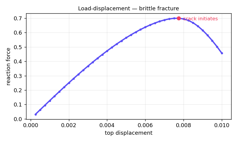
We pulled the top edge up in 40 steps on a 56×56 mesh. In most steps, little happens. The specimen stretches. The reaction rises almost linearly. The pre-notch is quiet. Then, near a top displacement of 0.008, the notch tip reaches its breaking energy. The crack runs.
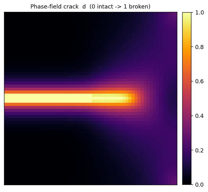
d. The sharp bright band is the crack. It grew straight across the specimen from the notch tip. The soft halo around it is the regularisation of the phase field. This "thickness" makes the discontinuity possible for finite elements.We did not prescribe that path. We put a notch on the left and pulled from the top. The energy competition produced the horizontal, mode-I crack. The force tells the other half of the story. It is the signature of brittle fracture: a near-linear rise to a peak, then a sudden drop as the crack cuts the specimen:
Why this is the hard case for an engine
Topology optimization was one physics in a loop. This is two physics in a loop. The same mesh must serve a vector structural problem and a scalar field problem. The element stiffness must scale for each element. The field solver must accept a reaction term that varies in space. physicsbase's Quad4 and FieldQuad4 are numerically verified separately against analytical references. Here they join with nothing between them but two arrays of numbers. That prior evidence narrows implementation risk; it does not prove the coupled fracture model physically adequate.
Honest footnotes
We used the standard AT2 phase-field model with a staggered solve. The references below and any modern fracture-mechanics course use this formulation. The code is our own. It reuses none of the published implementations. We used the simplest isotropic energy (no tension/compression split), a small mesh, and two staggered iterations per step. This is enough to reproduce the benchmark behaviour cleanly. It is not enough to reach the last few percent on the peak load, or to handle crack branching and compression-induced closure. The cited papers add those refinements: spectral energy splits, finer meshes, and monolithic or interior-point solvers. Our point was narrower. A general-purpose FE engine couples two of its own solvers through fields alone and grows the textbook crack.
References
- B. Bourdin, G. A. Francfort & J.-J. Marigo, "Numerical experiments in revisited brittle fracture," Journal of the Mechanics and Physics of Solids 48 (2000), 797–826.
- C. Miehe, M. Hofacker & F. Welschinger, "A phase field model for rate-independent crack propagation: Robust algorithmic implementation based on operator splits," Comput. Methods Appl. Mech. Engrg. 199 (2010), 2765–2778.
- Y. Bai et al., "An AsFem implementation for quasi-static brittle fracture phase field model" (2023). arXiv:2302.01510
- Interior-point methods for the phase-field approach to brittle and ductile fracture (2020). arXiv:2011.10125
examples/phasefield.py. It couples physicsbase's Quad4 and FieldQuad4 in one staggered loop. Read the docs →