physicsbase docs
This page gives an agent the complete simulation contract: author geometry or a finite-element model, assign materials and boundary conditions, solve, inspect the evidence, then change and re-submit the returned model. The same problem format supports one-time simulation, verification and optimization over REST, MCP, and the Python SDK.
Quickstart
A problem is a flat JSON object. It has nodes, materials,
elements, supports, and loads. Send it
to /v1/solve with POST. You get displacements, reactions, and element
stresses back. (No key yet? Send the same body to the keyless, size-limited
/demo/solve endpoint.)
# solve a single-bar problem
curl -X POST https://www.physicsbase.dev/v1/solve \
  -H "content-type: application/json" \
  -H "authorization: Bearer $PHYSICSBASE_KEY" \
  -d '{
    "nodes": [[0,0],[2,0]],
    "materials": {"steel": {"E": 200e9, "nu": 0.3}},
    "elements": [{"type":"truss2d","nodes":[0,1],
                  "material":"steel","section":{"A":0.01}}],
    "supports": [{"node":0,"dofs":["ux","uy"]},
                 {"node":1,"dofs":["uy"]}],
    "loads": [{"node":1,"fx":50000}]
}'ux = 5e-05 m. The support reacts with -50 kN. The
bar has 50 kN of tension. The system returns all of this as JSON.Authentication
Each solve needs an API key. Send it as a bearer token. Make a free key
on the sign-up page or with POST /auth/signup.
In the research preview there is no quota and no card. The discovery calls
(/capabilities, /health) are open.
authorization: Bearer pb_live_xxxxxxxxxxxxxxxxA missing key or a bad key returns 401. There is no solve quota
in the preview, but there is a fair-use rate limit (free plan: 60
solves/minute, 1,000/hour per key, 20,000 nodes per problem). Past it the
API returns 429 RATE_LIMITED with a Retry-After
header — sleep that many seconds and continue; for many problems use one
/v1/batch call. Oversize meshes return
413 PROBLEM_TOO_LARGE. Read your effective limits with
GET /auth/usage. Manage your keys and use data on your
account page.
The account console shows a 30-day solve history and manages named API keys. A
solve-scoped key can run solvers, imports and jobs; an
account-scoped key can read usage and create, edit, rotate or
revoke credentials. Use GET/POST /auth/keys,
PATCH/DELETE /auth/keys/{id}, and
POST /auth/keys/{id}/rotate. Full secrets are returned once,
only when created or rotated.
Long solves run as background jobs. A problem over ~5,000 nodes
gets HTTP 202 and a job_id instead of blocking the
connection. Poll GET /v1/jobs/{id} (free) until
status is done; the result is in the poll body. Use
POST /v1/jobs to force async for any size. CAD and large
/v1/import uploads put the entire import → mesh → solve
pipeline in the same job system. Use ?mode=sync to force
blocking. Details in the
API reference.
Repeated problems reuse verified results. A canonical problem hash drives a
bounded TTL/LRU cache shared across REST, MCP, async jobs, scalar fields, and the
in-process Python client. Concurrent duplicate misses coalesce to one solve and every
caller receives an isolated copy. summary.cache exposes hit/miss evidence;
failed solves are never stored.
How agents use it
The split of work is the important idea. The agent owns the design intent: it can create geometry or mesh connectivity, choose materials and sections, define supports, contacts, loads and analysis settings, or start from imported engineering data. physicsbase owns the numerical execution: model checks, meshing where needed, assembly, solution, result recovery and scoped verification evidence. The agent reads those computed results and decides what to do next.
solve → inspect
fields, checks and provenance → decide → change geometry, material, boundary
conditions or loads → submit the returned model again. Stop after one solve, use the
result as a verification gate, or continue as an optimization loop.3D results and convergence playback
Copilot opens every solved mesh in a 3D-first post-processor. True 3D solids,
shells, frames, trusses and CAD meshes keep their XYZ coordinates. Native 2D continuum
and plate meshes are embedded at z=0 and labelled as a 2D midsurface in 3D;
the display does not claim that a plane model has through-thickness solid physics.
Drag to orbit, shift-drag to pan, use the mouse wheel to zoom, or select isometric, XY, XZ and YZ cameras. The viewer draws only the exterior faces of tet/hex solids, adds mesh, support and load overlays, and lets you probe a node for its XYZ coordinate, current timeline value and final value.
record_iterations: true. CG, co-rotational Newton, steady Navier-Stokes
Picard and contact active-set solves return their computed nodal iterate at every
recorded step; structural transient solves return sampled time-step states. The
timeline plots relative residual when the algorithm defines one. A sparse direct
factorization has no iterates, so its two positions are explicitly called
initial and direct solution. Modal/buckling playback sweeps
phase and is labelled as mode animation, not convergence.API and SDK callers opt in with {"record_iterations": true,
"return_model": true}. The states are stored in
model.animation.frames; model.viewer describes the default
camera and interactions. Copilot keeps these large nodal arrays in the browser
visualization payload and out of the language-model context.
File-to-simulation
File import is optional. When geometry or an FE model already exists, the agent can skip manual mesh
transcription. Send {filename, content_base64} to
POST /v1/import, or call MCP fem_import with a local
path or uploaded content. STEP/STP/IGES/BREP geometry is meshed by
gmsh/OpenCASCADE. Abaqus INP is read natively; Nastran, Gmsh, VTK/VTU,
MED, STL/OBJ/PLY and other mesh formats use meshio.
Raw CAD contains shape, not analysis intent, so include a material plus
supports and loads. Select nodes by explicit index, named node set, or a
coordinate plane such as {"axis":"x","op":"min"}. The response
is the normal solved result plus a complete model bundle. Its import manifest
records the source SHA-256, adapter and meshing settings, coordinate scale, element counts,
named sets, and any quadratic-cell linearisation warnings.
202. Poll the supplied URL; when it says done,
result.model is the completed simulation ready to inspect,
animate, download, or re-submit. Unsupported Abaqus physics/assembly cards
fail explicitly rather than producing a silently incomplete model.One-call CAD quickstart
For CAD/LLM integrators there is a single call that takes a geometry file
plus plain intent — a material name, what to clamp, what to push — and
returns a meshed, solved, verified result. No mesh API, no material
constants, no DOF bookkeeping. Use mesh_cad first to inspect
node/element counts and pick a budget, then simulate_cad.
from femengine.client import FEMClient
client = FEMClient()                       # in-process; or FEMClient(base_url=…) for remote

# 1. Inspect the mesh before committing to a solve
info = client.mesh_cad("bracket.step", target_nodes=20000)
info["stats"]["n_nodes"], info["element_breakdown"]

# 2. Mesh + solve + verify in one call
out = client.simulate_cad(
    "bracket.step",
    material="aluminum_6061",           # library name or {"E","nu","rho"}
    fix={"largest_face": True},        # auto-pick the big flat face to clamp
    load={"face": "z_max", "fz": -5000}, # 5 kN total, downward
    target_nodes=20000)
out["summary"]["verification"]["verdict"]["status"]  # PASS / REVIEW / …
The same flow is available over HTTP at POST /v1/import
(add "mesh_only": true for the inspect step) and as the MCP tools
fem_cad_mesh / fem_cad_solve, which also accept a
local path or a base64 content upload.
| Concern | How you say it |
|---|---|
| Material | "aluminum_6061", "steel", "ti64"… (GET /materials lists the library) or a raw {"E","nu","rho"}; override a library value with {"library":"steel","rho":7900}. |
| What to clamp / load | A selector: {"face":"z_min"} (or top/bottom/left…), {"largest_face":true}, {"bbox":[…]}, {"sphere":{"center","radius"}}, {"surface":"MOUNT"} for a preserved CAD name, {"cad_face":12} for a stable face tag returned by mesh_cad, or {"all":true}. A load adds a force component (fx/fy/fz, total newtons). |
| Mesh size | resolution = coarse|medium|fine|very_fine, a target_nodes budget (auto-coarsens to stay tractable), or an explicit mesh_size. |
summary.verification. Numerical
verification (equilibrium, mesh quality, discretization estimate) is not the
same as physical validation — read the verdict and refine before any
design-release decision.Run the packaged STEP examples
The homepage's first problem is not browser-generated mesh JSON. It calls
POST /demo/cad/uav-wing-gust with a bounded load_n,
reads the hash-pinned swept-wing STEP, meshes it with gmsh/OpenCASCADE,
maps an elliptical lift law to area-weighted upper-surface nodal forces,
and returns the completed model bundle. The catalog also includes the NASA
CRM wing envelope and original 2020-corner-bracket examples.
GET /demo/cad returns source, author, usage/license,
geometry/derivative disclosure, load range and model, material, and mesh
policy. The keyless route is rate-limited and never accepts a path or file
upload.
curl -X POST https://www.physicsbase.dev/demo/cad/uav-wing-gust \
  -H "content-type: application/json" \
-d '{"load_n":4000}'summary.verification: equilibrium and mesh quality are
checked, while the stress-recovery estimate can return REVIEW and
request refinement before a design-release decision. The NASA example is a
transparent scale-matched solid envelope, not the exact outer mold line,
internal wing structure, manufacturing drawing, flight article, or
certification evidence. Read the full case
study → The UAV case is likewise an equivalent-solid concept, not a
laminate or internal wing-box. Read the
distributed-gust case →Automotive explicit-dynamics evidence
GET /demo/automotive exposes a checksum-verified
2.277-million-element CCSA Camry reference and the OpenRadioss backend
contract. It is a read-only evidence catalog: it does not launch a crash
job from a web request. The full Camry run is explicitly marked pending an
adequately provisioned persistent worker; published CCSA/LS-DYNA force,
crush and validation data remain labelled as external evidence.
Agent guide: the reliable loop
Do these five steps. Then the first call is correct. Each step names the field or the tool to use.
| # | Step | How |
|---|---|---|
| 1 | Discover | Call fem_capabilities (MCP) or GET /capabilities. It returns the element types, DOF names, load components, and analyses. Read them. Do not guess. |
| 2 | Pick the element | Use the table below to match the physical problem to a type. All elements in a model must use the same DOF layout. Examples are all 2D-planar or all 3D. |
| 3 | Build the JSON | Fill nodes, materials, elements, supports, and loads. Add enough supports to stop all rigid-body motion. |
| 4 | Call | fem_solve / fem_modal / fem_buckling, or POST to /v1/solve with "analysis" set. |
| 5 | Read and act | Read displacements, reactions, and elements[]. Look at the error contract first. A returned {"error": …} tells you what to correct. |
How to choose an element and analysis
| The problem is… | Use | Analysis |
|---|---|---|
| Pin-jointed truss (2D) | truss2d | static |
| Space truss (3D) | truss3d | static |
| Beam / portal frame (2D bending) | beam2d | static |
| 3D frame, torsion, biaxial bending | frame3d | static |
| Panel / bracket / plane part | quad4 or cst | static |
| Vibration — natural frequencies | any (needs rho) | modal |
| Column / frame stability | beam2d / frame3d | buckling |
A full agent transcript
This shows what an MCP agent does from start to end. It answers the question "Is my 3 m cantilever safe with a 5 kN tip load?".
# 1. discover — learn the schema before building anything
→ fem_capabilities()
← { "element_types": { "beam2d": "…section {A, I}", … }, "analyses": [ … ] }

# 2+3. translate the words into a problem and solve
→ fem_solve({
    "nodes": [[0,0],[1,0],[2,0],[3,0]],
    "materials": { "steel": { "E": 210e9, "nu": 0.3 } },
    "elements": [
      {"type":"beam2d","nodes":[0,1],"material":"steel","section":{"A":0.01,"I":8e-6}},
      {"type":"beam2d","nodes":[1,2],"material":"steel","section":{"A":0.01,"I":8e-6}},
      {"type":"beam2d","nodes":[2,3],"material":"steel","section":{"A":0.01,"I":8e-6}}
    ],
    "supports": [ {"node":0,"dofs":["ux","uy","rz"]} ],
    "loads": [ {"node":3,"fy":-5000} ]
  })
← { "displacements": [ …, {"uy": -0.0268, "rz": -0.0134} ],
    "reactions": [ {"fy": 5000, "mz": 15000}, … ],
    "elements": [ {"moment_i": 15000, …}, … ] }

# 4. reason on the returned numbers (no physics guessed by the agent)
tip_drop = 26.8 mm            # from displacements[-1].uy
M_wall   = 15 kN·m            # from reactions[0].mz / elements[0].moment_i
sigma    = M_wall * c / I = 94 MPa
verdict = 94 MPa < 250 MPa yield -> safe, factor of safety 2.7Error contract and troubleshooting
The engine gives clear and specific errors. On MCP a bad problem returns
{"error": "…"}. It never returns a stack trace. On REST it returns
422 with a detail string. You can act on both messages
directly. These are the common causes:
| Message contains… | Cause | Correction |
|---|---|---|
| no supports; stiffness is singular | The structure can move or turn freely. This is rigid-body motion. | Add supports to stop all rigid-body modes. Or add springs. |
| unknown element type | The type is wrong or not supported. | Use one of truss2d, truss3d, beam2d, frame3d, cst, quad4. |
| needs N nodes, got M | The element has the wrong number of nodes. | truss/beam = 2, cst = 3, quad4 = 4, frame3d = 2. |
| is 3D but model is 2D (or vice-versa) | The model mixes 2D and 3D elements. Or the coordinate count is wrong. | Use one dimension only. Give 3D nodes three coordinates. |
| support dof '…' invalid | You used a DOF that the model does not have. An example is rz in a truss-only model. | See dof_names from /capabilities. A 2D truss has ux,uy. Add a beam2d for rz. A frame3d has all six. |
| load component '…' not valid | You applied a component such as mz where there is no rotational DOF. | Apply only the components that the model has. Moments need beam or frame elements. |
| has no mass matrix (modal) | You ran modal without rho. | Give each material a rho that is not zero. |
| no axial force … nothing to buckle | You ran buckling with no compression in any member. | Apply an axial compression load along the members. |
| element references node N out of range | A node index is more than the nodes list. | Node indices start at 0. Keep them < len(nodes). |
7e-12 are floating-point zero. If a reaction on a
free node is large, a support or a connection is wrong.Problem schema
Coordinates are [x, y] for 2D models or [x, y, z]
for 3D. Node indices start at 0. They point to positions in the
nodes array. The units are SI in and SI out. Give metres
and newtons. You get metres and newton-metres back.
| Field | Type | Description |
|---|---|---|
nodes | number[][] | List of coordinates, 2D or 3D. |
materials | object | Named map of {E, nu, rho?} (Young's modulus, Poisson's ratio, density). |
elements | object[] | {type, nodes, material, section, id?} — see the element reference. |
supports | object[] | {node, dofs, values?}. DOFs: ux, uy, uz, rx, ry, rz. values prescribes non-zero displacement. |
loads | object[] | {node, fx?, fy?, fz?, mx?, my?, mz?} — nodal forces and moments. |
element_loads | object[] | {element, w:[wx,wy(,wz)]} — distributed load (force/length) on a beam or frame element. |
springs | object[] | {node, dof, k} — grounded elastic support of stiffness k. |
gravity | number[] | [gx, gy(, gz)] — acceleration vector for self-weight (needs rho). |
analysis | string | "static" (default), "modal", or "buckling". |
title | string | Optional label echoed back in the summary. |
Element reference
Choose an element family with type. The section keys
are different for each family.
| type | DOF / node | section | Use for |
|---|---|---|---|
truss2d | ux, uy | A | 2D bars / pin-jointed trusses |
truss3d | ux, uy, uz | A | 3D space trusses |
spring | ux, uy | k | Spring assemblages, elastic links |
beam2d | ux, uy, rz | A, I | 2D frames, beams, Euler-Bernoulli bending |
timo2d | ux, uy, rz | A, I, ks? | Timoshenko beam — includes shear (deep beams) |
frame3d | ux…rz (6) | A, Iy, Iz, J, G?, ref? | 3D frames: axial + torsion + biaxial bending |
plate4 | uz, rx, ry | t, ks? | Reissner-Mindlin plate bending |
cst | ux, uy | t, kind | 2D continuum, linear triangle |
quad4 | ux, uy | t, kind | 2D continuum, bilinear quad |
tri6 | ux, uy | t, kind | 2D continuum, quadratic triangle (LST) |
quad8 | ux, uy | t, kind | 2D continuum, 8-node serendipity quad |
tet4 | ux, uy, uz | — | 3D solid, linear tetrahedron |
hex8 | ux, uy, uz | — | 3D solid, trilinear hexahedron |
tet10 | ux, uy, uz | — | 3D solid, quadratic tetrahedron (10-node) |
hex20 | ux, uy, uz | — | 3D solid, serendipity hexahedron (20-node) |
mitc4 | uz, rx, ry | t, ks? | MITC4 plate — assumed strain, locking-free, rank-sufficient |
shell_mitc4 | ux…rz (6) | t | Flat shell with MITC4 bending (locking-free) |
axiquad4 | ur, uz | — | Axisymmetric solid (r-z plane) |
For cst and quad4, t is the thickness.
kind is "plane_stress" (the default) or
"plane_strain". Give the quad4 nodes in counter-clockwise
order. For frame3d, Iy and Iz are the second
moments about the local y and z axes. J is the torsion constant.
G has the default E/2(1+ν). ref is an
optional orientation vector for the cross-section. It has a sensible default. It
changes to global Y for vertical members.
Result schema
Each solve returns the same shape. Thus an agent can read it directly.
{
  "displacements": [ { "ux": 0.0, "uy": 0.0 }, … ],   // per node, by DOF
  "reactions":     [ { "fx": -50000.0, "fy": 0.0 }, … ], // per node
  "elements": [
    { "id": "span_1", "type": "beam2d",
      "moment_i": 10000.0, "shear_i": 5000.0, … }  // depends on type
  ],
  "summary": { "n_dof": 9, "max_abs_displacement": 0.0079,
                "solve_ms": 1.2 }
}
The element results change with the family. Trusses return axial_force and
axial_stress. Beams return shear_i/j and
moment_i/j. Continuum elements return a stress vector
and von_mises. Treat values such as 7e-12 as
floating-point zero.
REST API
POST/solve solves a problem.
GET/capabilities gives the element
types and DOF names. GET/health
shows that the service is available.
const res = await fetch("https://www.physicsbase.dev/v1/solve", {
  method: "POST",
  headers: { "content-type": "application/json" },
  body: JSON.stringify(problem)
});
const out = await res.json();
console.log(out.displacements.at(-1).uy); // tip deflection
MCP server
You can give a solver as direct tools to any MCP agent, such as Claude.
The server gives eight tools: fem_capabilities,
fem_example, fem_solve (static),
fem_modal (frequencies), fem_buckling
(critical loads), fem_transient, fem_damage, and
fem_field (heat, diffusion, and flow).
Remote (recommended). The deployed service hosts MCP over
streamable HTTP at /mcp. Thus a client connects by URL. You
install nothing and need no key:
// MCP client config — remote endpoint
{
  "mcpServers": {
    "physicsbase": {
      "url": "https://www.physicsbase.dev/mcp"
    }
  }
}
Local (stdio). Or run the server as a subprocess:
{
  "mcpServers": {
    "physicsbase": {
      "command": "python",
      "args": ["-m", "femengine.mcp.server"]
    }
  }
}
The agent calls fem_capabilities one time to learn the schema. Then
it sends a problem object to fem_solve. It gets the results
JSON as the tool response.
Use it in ChatGPT
The plain browsing tool of ChatGPT is read-only. It can read this page but
it cannot POST to /v1/solve. To let ChatGPT call the solver,
add physicsbase as a GPT Action. This takes about one minute. There is
no key to set:
- In ChatGPT, go to Explore GPTs → Create. Then open the Configure tab.
- Under Actions, click Create new action.
- Click Import from URL. Paste the OpenAPI schema URL:
https://www.physicsbase.dev/openapi.json - Set Authentication to None. physicsbase needs no key.
- Save. Your GPT now has
solve,modal,buckling,transient,damage, andfieldas operations that it can call.
Use a system prompt like this for the GPT: "You are an FEA assistant. Call GET /capabilities first to learn the valid element types and DOFs. Then POST /solve with a JSON problem. Report the displacements, reactions, and stresses from the response of the solver. Do not compute them yourself."
/openapi.json. Claude and other MCP clients connect directly to
the remote endpoint at https://www.physicsbase.dev/mcp. See
the MCP server section above.Python SDK
Build models in code, or solve a JSON spec. With no base_url the
client solves in the same process. This is useful for tests and local agents.
Give a URL to call a running server.
from femengine import Model, solve
from femengine.materials import Material
from femengine.client import FEMClient

# fluent model builder
m = Model()
m.add_nodes([[0,0], [2,0]])
m.add_material("steel", Material(E=200e9, nu=0.3))
m.add_element("truss2d", [0,1], "steel", {"A": 0.01})
m.add_support(0, ["ux","uy"]); m.add_support(1, ["uy"])
m.add_load(1, fx=50_000)
res = solve(m)
print(res.displacements[1]["ux"])   # 5e-05

# …or solve a JSON spec via the client
out = FEMClient().solve(problem_dict)          # in-process
out = FEMClient("https://www.physicsbase.dev").solve(problem_dict)
Advanced analyses
The engine also solves two eigenvalue problems. Set
"analysis" in the problem. Or call the special endpoints
(/modal, /buckling) and MCP tools.
Modal — natural frequencies
This solves (K − ω²M) φ = 0 with consistent mass matrices. The materials
must include rho. The system ignores applied loads. It returns
frequencies_hz, angular_frequencies, and normalised
mode_shapes (for each node and each DOF).
{
  "frequencies_hz": [ 4.79, 30.0, 84.1, … ],
  "angular_frequencies": [ 30.1, 236.5, 528.3, … ],
  "mode_shapes": [ [ {"ux":0.0,"uy":0.0,"rz":0.0}, … ], … ],
  "summary": { "num_modes": 6, "analysis": "modal" }
}
Buckling — critical loads
This runs a reference static solve. It forms the geometric stiffness from the member
axial forces. Then it solves (K + λ Kg) φ = 0. The applied
loads give the reference pattern. The load_factors multiply that
pattern to reach buckling. The critical_loads give the absolute
magnitudes. The result agrees with Euler columns to about 1%.
3.4 means that the
structure buckles at 3.4 times the load that you applied. A factor below 1 means that the
applied load is already more than the critical load.Multiphysics
physicsbase also solves scalar-field problems. It uses one
kernel for all of them. The governing equation is
−∇·(k∇u) + v·∇u = Q. The meaning of u, k, and
Q selects the physics.
| Physics | u | k | Notes |
|---|---|---|---|
| Heat conduction | temperature | conductivity | source = heat generation; c = ρ·cp for transient |
| Mass diffusion | concentration | diffusivity | Fick's law; identical math |
| Potential flow | velocity potential | 1 | inviscid, irrotational; ∇u = velocity |
| Seepage / Darcy | hydraulic head | permeability | groundwater flow |
| Transport | concentration | diffusivity | set velocity → convection-diffusion |
The field elements are field_line2 (1D), field_tri3,
field_quad4 (2D), field_tet4, and field_hex8
(3D). Each node has one DOF, the scalar. The boundary conditions are a prescribed
value (Dirichlet), a flux (Neumann), and a
convection (Robin: q = h(u − u∞)). The solve is steady or
transient (the θ-method). Call POST /field or the
fem_field MCP tool.
Heat conduction with a source
A 1D bar has uniform heat generation and cold ends. It gets a parabolic
temperature profile. The peak is Q L² / 8k.
{
  "nodes": [[0],[0.25],[0.5],[0.75],[1]],
  "materials": { "steel": { "k": 45 } },   // W/m·K
  "elements": [ /* field_line2 chain */ ],
  "element_sources": [ /* {element:i, Q:1e5} heat gen per element */ ],
  "values": [ {"node":0,"value":20}, {"node":4,"value":20} ]
}
// -> { "values": [20, …, T_mid, …, 20], "fluxes": [ … ] }
Potential flow and transport
With k = 1 and no source, the field solves the Laplace equation. This gives a velocity
potential. Its gradient is the flow field. Add a velocity and
the same solver does convection-diffusion transport. This is a scalar that a
flow carries. The result agrees with the analytical boundary-layer profile
(e^{Pe·x} − 1)/(e^{Pe} − 1) at a low Péclet number.
{
  "nodes": [ /* 1D chain 0 … 1 */ ],
  "materials": { "m": { "k": 1.0 } },   // diffusivity D
  "elements": [ /* field_line2 */ ],
  "velocity": [1.0],                     // advection speed
  "values": [ {"node":0,"value":0}, {"node":-1,"value":1} ]
}
Coupled thermo-mechanical
This is true multiphysics. It solves the heat field. It maps the nodal temperatures onto the
structure as a ΔT for each element. Then it solves for the thermal stress. It does all of this
in one call. A fully restrained bar at temperature T returns
σ = −Eα(T − T_ref).
from femengine import thermo_mechanical

res = thermo_mechanical(field_model, struct_model, T_ref=20.0)
res.structural["elements"][0]["axial_stress"]   # thermal stress
res.element_dT                                  # ΔT applied per element
For a two-way loop, thermo_mechanical_twoway lets the mechanical
deformation feed back into the heat problem: element conductivity follows
k_eff = k0·(1 + β·tr(ε)), and the two solves are iterated to a
self-consistent fixed point. β = 0 recovers the one-way solve
exactly; the return carries a convergence self-check (iterations and
temperature residual).
from femengine.coupling import thermo_mechanical_twoway

res = thermo_mechanical_twoway(field_model, struct_model, beta=3e-3, T_ref=20.0)
res["summary"]["verification"]["converged"]   # fixed point reached
res["summary"]["verification"]["iterations"]
Nonlinear damage
This is continuum isotropic damage. The stiffness goes down as
σ = (1 − d)·D:ε. It has exponential softening after a threshold
strain. The system applies the load in steps with a secant iteration. Use
prescribed displacements to follow the softening branch.
{
  "analysis": "damage", "k0": 1e-4, "kf": 5e-4, "increments": 30,
  "nodes": [[0,0],[1,0]],
  "materials": { "concrete": { "E": 30e9, "nu": 0.2 } },
  "elements": [ {"type":"truss2d","nodes":[0,1],"material":"concrete","section":{"A":0.01}} ],
  "supports": [ {"node":0,"dofs":["ux","uy"]},
                 {"node":1,"dofs":["ux","uy"],"values":[3e-4,0]} ]
}
// -> { "history":[{load_factor,max_damage,…}], "elements":[{damage,…}] }analysis: stokes, verified vs Poiseuille), steady
Navier-Stokes with convection via Picard/Oseen (analysis: navier_stokes,
verified vs Kovasznay), and transient Navier-Stokes via backward-Euler time
stepping (analysis: unsteady_navier_stokes, verified vs the exact
Taylor-Green vortex decay). Turbulence models, free-surface flow and
fluid-structure interaction are on the roadmap; we do not claim them now.Run it locally
The engine is a complete Python package (NumPy and SciPy). You can run the solver directly. Or you can start the REST API. Or you can give it over MCP.
Install
cd fem-engine
pip install -e ".[api,mcp,dev]"      # API includes meshio + gmsh for CAD import
Headless Debian/Ubuntu deployments also need the system packages
libgl1 libglu1-mesa libxrender1 libxcursor1 libxfixes3 libxext6
      libxft2 libfontconfig1 libxinerama1 libx11-6 libgomp1 zlib1g libstdc++6
      libgcc-s1
so the gmsh native runtime can load its complete direct
non-glibc dependency set, including the headless X11 libraries.
Railway deployments include the set through the repository's
railpack.json.
Solve in Python (no server)
from femengine import Model, solve
from femengine.materials import Material

m = Model()
m.add_nodes([[0,0], [3,0]])
m.add_material("steel", Material(E=210e9, nu=0.3))
m.add_element("beam2d", [0,1], "steel", {"A":0.01, "I":8e-6})
m.add_support(0, ["ux","uy","rz"])
m.add_load(1, fy=-5000)
print(solve(m).displacements[-1])      # tip deflection
Start the REST API
femengine-api --port 8000                 # or: uvicorn femengine.api.server:app

curl -s localhost:8000/capabilities        # discover elements & analyses
curl -s -X POST localhost:8000/v1/solve \
     -H "content-type: application/json" \
     -d @examples/cantilever_beam.json         # solve a saved problem
The interactive API docs are at localhost:8000/docs.
The endpoints are /solve, /modal, /buckling,
/transient, /capabilities, and /health.
Expose it over MCP
python -m femengine.mcp.server               # tools: fem_solve, fem_modal,
                                             # fem_buckling, fem_transient, …
Numerical verification and tests
Do not trust the engine on faith. The system checks each element and analysis against a closed-form solution. The test suite is the specification. If a value from the engine does not match the textbook answer within the tolerance, the test fails.
Run the suite
cd fem-engine
pytest -q                     # all suites
pytest tests/test_validation.py -q     # core elements
pytest tests/test_advanced.py -q       # 3D frames, modal, buckling
pytest tests/test_textbook.py -q       # solids, thermal, axisym, transient
What each check proves
| Suite | Reference checked |
|---|---|
test_validation.py | Axial bar PL/AE, symmetric truss equilibrium, cantilever tip PL³/3EI and rotation ML/EI, CST/Quad4 uniaxial tension, 3D bar. |
test_advanced.py | 3D frame bending about both axes + torsion TL/GJ, UDL deflections wL⁴/8EI & 5wL⁴/384EI, self-weight bar, spring, cantilever & simply-supported natural frequencies, Euler buckling (pinned, cantilever, fixed-fixed). |
test_textbook.py | Spring assemblage, restrained/free thermal bar −EαΔT, uniform-strain patch tests for tri6/quad8/tet4/hex8/axiquad4, hex8 uniaxial, edge traction, body force, undamped step-response 2× overshoot. |
test_multiphysics.py | Heat conduction (linear, parabolic source QL²/8k, convection, flux BC), 2D/3D field patch tests, transient→steady, potential flow, convection-diffusion boundary layer, coupled thermal stress, and the nonlinear damage law. |
test_roadmap.py | Unilateral contact (bar-into-stop force kg−P, no-penetration release); co-rotational geometric nonlinearity vs the exact von Mises snap-through; Crisfield arc-length tracing the full path through the limit point; the Scordelis-Lo shell roof converging to 0.3024; and Hertzian contact recovering the pressure ellipse (half-width & peak within 0.3%); and finite-strain Neo-Hookean hyperelasticity matching the exact uniaxial rubber stress, mesh-independently; and steady-state harmonic response matching the exact SDOF transfer function with the resonance peak on the modal frequency; and Coulomb friction holding a block until tan θ crosses μ; and a multi-step load/unload/reload history carrying the exact plastic permanent set between steps. |
test_api.py | REST endpoints, capability discovery, error handling, MCP tool round-trip. |
How the system verifies the numbers
The pattern is the same in all tests. Build a problem with a known closed-form answer. Solve it. Then check that the result equals the answer within the tolerance.
def test_buckling_pinned():
    m, p = _column("pinned")              # pin-ended steel column
    res = buckling(m, num_modes=1)
    expected = math.pi**2 * p["E"] * p["I"] / p["L"]**2   # Euler's Pcr
assert res.critical_loads[0] == pytest.approx(expected, rel=1e-2)pytest -q and python -m verification.suite to reproduce it.Each solve checks itself
The offline suite shows that recorded implementation claims reproduce their references within
their thresholds. It does not prove the engine correct for every use. An agent must also inspect
the numerical quality of one solve, including whether the mesh is fine enough. Every analysis therefore returns a scoped verification
block with checks_run, checks_not_run, numerical values and tolerances,
and a PASS, REVIEW, FAIL, or NOT_CHECKED verdict. Static solves add
global equilibrium, mesh quality, and a recovery-based discretization-error estimate
(Zienkiewicz-Zhu). The estimator marks a coarse mesh; it never returns a false
“converged”.
Other analyses check their own governing equations: modal and buckling eigenpair residuals;
transient and harmonic dynamic equilibrium; Richardson time-step accuracy for linear
Newmark and scalar-field transients; nonlinear equilibrium and Newton convergence;
contact complementarity and Coulomb admissibility; viscoelastic/creep equilibrium; and scalar-field
residuals. These prove solution quality for the discrete equations. They do not pretend to prove mesh,
time-step, or model-form accuracy; missing estimators are named under checks_not_run.
Contact analyses can additionally run a real two-grid sensitivity study. Set
estimate_contact_error:true and physicsbase solves a one-level
uniformly refined supported mesh, returns that refined model, and compares total
and per-contact force, penetration/gap violation, and active-set stability. A
positive contacts[].contact_area adds pressure convergence. The
evidence is returned under summary.contact_convergence and copied into
model.self_check.contact_convergence. This is one-level sensitivity,
not an asymptotic bound or a large-sliding/surface-to-surface claim.
The static discretization-error estimate covers supported continuum families. This includes plane stress and plane strain continuum, 3D solids (tet4 and hex8, with an energy norm over the six-component stress), Mindlin plates (an energy norm over the bending moments), and flat shells (the membrane component). The system groups the recovery by element family. Thus it averages only compatible stress measures at a shared node. We test the estimator behavior explicitly. A constant-stress state estimates about 0 error at any resolution. A real gradient estimates less error as the mesh gets finer.
If the verdict is REVIEW because the mesh is too coarse, the engine can correct
it for you. Set analysis: "adaptive". The engine makes the quad mesh finer and solves
again. It repeats this until the estimated error is below target_error. It returns the
converged result and the full refinement history (elements, DOF, and error for each round). This is
the verifier that also corrects the mesh.
Refinement works in one of two ways. The default is refine_strategy: "uniform". It splits
every quad each round. This is conforming and monotone. It is the reliable choice for the convergence
decision. refine_strategy: "adaptive" is targeted. A Dörfler marking step refines only
the elements that carry the error. Constraints tie the hanging nodes on the coarse-fine interface. The
constraints use linear interpolation. This gives similar accuracy with far fewer elements when the
error is local. Examples are stress concentrations and re-entrant corners. We verify the hanging-node
constraint against the FE patch test. A refined element next to a coarse element still reproduces a
linear field exactly. It carries continuous stress across the junction.
{ "balanced": true, "relative_residual": 2.1e-16,
  "discretization_error": { "percent": 0.9, "converged": true,
                            "method": "Zienkiewicz-Zhu stress recovery" },
  "mesh_quality": { "max_aspect_ratio": 1.8, "inverted_elements": 0, "acceptable": true },
  "verdict": { "status": "PASS", "reasons": [] } }
The verifier answers the question “Can I trust these numbers?” The assessment answers the
next question: “Is the part OK?” Each static solve also returns
summary.assessment. It gives the peak von Mises stress and its location. It gives the peak
deflection and its location. It gives the safety factor against an allowable_stress
(for each material or for the whole problem). It gives a deflection check against allowable_deflection. It gives a
PASS, FAIL, or REVIEW verdict. If you give
no limit, it reports REVIEW with the raw numbers. It does not give a false pass. Thus
an agent gets a decision to act on, not a field to interpret.
{ "status": "PASS",
  "max_von_mises":   { "value": 1.8e8, "unit": "Pa", "element": 3, "location": [0.25, 0.13] },
  "max_displacement": { "magnitude": 0.0094, "unit": "m", "node": 84, "location": [8.0, 0.0] },
  "safety_factor": { "value": 1.39, "allowable_stress": 2.5e8, "status": "PASS" },
  "deflection_check": { "max_displacement": 0.0094, "allowable": 0.02, "status": "PASS" },
"headline": "PASS: peak von Mises 1.8e8 Pa at [0.25, 0.13]; peak deflection 0.0094 m at node 84; SF 1.39" }Analytical and legacy target reproductions
The cases below are useful implementation regressions, but they are not all complete qualification studies and none is physical validation. For release-level published targets, fixed acceptance rules, mesh histories, formulation deviations, and failures, use the Benchmark Guide.
| Benchmark | What it tests | Result |
|---|---|---|
| Scordelis-Lo roof (MacNeal & Harder, 1985) | Membrane-bending shell accuracy — shell4 | free-edge deflection converges to 0.3024 (0.0% at 16×16, monotone from below). Read the post → |
| Hertzian contact (Hertz, 1882) | Exact active-set contact, elliptic pressure — analysis: contact | contact half-width & peak pressure within 0.3%; profile follows p₀√(1−(x/a)²). Read the post → |
| von Mises snap-through | Geometric nonlinearity — analysis: nlgeom | reaction matches the exact P(w) to 1e−6 through the sign flip. Read the post → |
| Arc-length limit point (Crisfield / Riks) | Continuation past the limit point — analysis: arclength | traces the full snap-through path (which load control cannot cross) to 1e−15. Read the post → |
| Neo-Hookean uniaxial (finite strain) | Large-deformation continuum, Newton-Raphson — analysis: hyperelastic | Cauchy stress matches the exact rubber solution to machine precision; Newton converges quadratically. |
| SDOF frequency response (harmonic) | Forced steady-state response with damping — analysis: harmonic | amplitude matches the exact transfer function to machine precision; the resonance peak sits on the modal frequency. |
| Block on an incline (Coulomb friction) | Stick vs slip on a contact interface — analysis: friction | normal and tangential reactions exact; the interface holds if and only if tan θ ≤ μ, to machine precision. |
| Elastoplastic load / unload / reload (multi-step) | State carried across steps — analysis: steps | the exact 1D elastoplastic path, permanent set and residual stress carried forward between steps. |
| Off-axis composite lamina (Jones / CLT) | Orthotropic plane-stress stiffness & shear-extension coupling | recovered stress equals the transformed Q̄(θ)·ε to machine precision, over 120 lamina cases. |
| Composite laminates & failure (CLT / Hashin / Thiele) | ABD stiffness, homogenization, ply-failure, oxidation | plate stiffness, rule-of-mixtures, first/last-ply-failure at Yt/Xt, and the Thiele oxidation profile — all exact (58 cases). |
| Composite literature (Tsai-Pagano / Tsai-Wu / WWFE) | Quasi-isotropic invariants, failure criterion, WWFE lamina | quasi-isotropic modulus (U1²−U4²)/U1 and Tsai-Wu axis strengths reproduced to machine precision. Case study → |
Textbook coverage
The engine covers the finite-element topics in a standard undergraduate and graduate structural-mechanics course. Each row is a topic and the capability that solves it.
| Curriculum topic | Capability | Status |
|---|---|---|
| Direct stiffness & spring assemblages | spring | ✓ |
| Bars & trusses (2D / 3D) | truss2d, truss3d | ✓ |
| Beams & plane frames | beam2d | ✓ |
| Space frames, grids (torsion, biaxial bending) | frame3d | ✓ |
| Distributed loads & equivalent nodal loads | element_loads | ✓ |
| Plane stress / plane strain, linear | cst, quad4 | ✓ |
| Higher-order plane elements (LST, Q8) | tri6, quad8 | ✓ |
| Isoparametric formulation & Gauss quadrature | quad4/quad8/hex8 | ✓ |
| 3D solids (tetrahedra, hexahedra) | tet4, hex8 | ✓ |
| Axisymmetric solids | axiquad4 | ✓ |
| Thermal stress / thermal loads | thermal + material alpha | ✓ |
| Body forces & surface tractions | body_forces, tractions | ✓ |
| Self-weight (gravity) | gravity | ✓ |
| Supports: pinned/fixed/roller, settlement, elastic | supports, values, springs | ✓ |
| Statically indeterminate structures | direct global solve | ✓ |
| Dynamics: natural frequencies & mode shapes | modal (consistent mass) | ✓ |
| Transient response (time integration) | transient (Newmark) | ✓ |
| Elastic stability / linear buckling | buckling (geometric stiffness) | ✓ |
| Heat conduction (steady + transient) | field + field_* elements | ✓ |
| Mass diffusion (Fick) | field (same kernel) | ✓ |
| Convection / Robin boundaries | convections | ✓ |
| Convection-diffusion transport | field + velocity | ✓ |
| Potential (inviscid) flow, seepage | field, k=1 | ✓ |
| Coupled thermo-mechanical | thermo_mechanical | ✓ |
| Nonlinear continuum damage | damage | ✓ |
| Shear-deformable (Timoshenko) beams | timo2d | ✓ |
| Plate bending (Reissner-Mindlin) | plate4 | ✓ |
| Elastoplasticity (von Mises / J2) | plasticity | ✓ |
| Linear-elastic fracture, K₁ (XFEM) | examples/xfem.py | ✓ |
| Flat shell (membrane + bending) | shell4 | ✓ |
| Geometric nonlinearity (large displacement) | analysis: nlgeom | ✓ |
| Contact: barriers, deformable pairs, node-to-surface + opt-in two-grid spatial convergence | analysis: contact | ✓ |
| Finite-strain hyperelasticity (Neo-Hookean, Mooney-Rivlin, Ogden, transversely isotropic + GOH dispersion fibre) | analysis: hyperelastic | ✓ |
| Steady-state (harmonic) dynamics / frequency response | analysis: harmonic | ✓ |
| Frictional contact (Coulomb stick/slip) | analysis: friction | ✓ |
| Multi-step load history (load / unload / reload) | analysis: steps | ✓ |
| Orthotropic / composite lamina (plane stress) | material {E1,E2,nu12,G12} + section angle | ✓ |
| Laminate ABD stack-up (classical lamination theory) | POST /laminate | ✓ |
| Micromechanics homogenization (fibre/matrix, woven) | POST /homogenize | ✓ |
| Progressive ply-failure (Hashin, first/last-ply) | POST /progressive_failure | ✓ |
| Oxidation reaction-diffusion (Thiele) | POST /oxidation | ✓ |
| Pluggable user material (UMAT hook) | section umat + registered law | ✓ |
| Adaptive auto-refinement (verifier fixes the mesh) | analysis: adaptive | ✓ |
| Higher-order 3D solids (quadratic tet, serendipity hex) | tet10, hex20 | ✓ |
| Assumed-strain plate/shell (MITC4, locking-free, rank-sufficient) | mitc4, shell_mitc4 | ✓ |
| Topology optimization (SIMP compliance minimization) | analysis: topology | ✓ |
| Fracture — stress-intensity factor (XFEM edge crack) | analysis: xfem | ✓ |
| Brittle fracture (phase-field, crack growth) | analysis: phasefield | ✓ |
| Moving heat source / melt pool (Rosenthal) | analysis: moving_heat | ✓ |
| Stress-stiffened (prestressed) modal analysis | analysis: prestress_modal | ✓ |
| Damped modal (complex eigenvalues, Rayleigh damping ratios) | analysis: damped_modal | ✓ |
| Gyroscopic rotor modes and Campbell critical speeds | analysis: rotordynamics | ✓ |
| Native explicit dynamics (linear elements; nonlinear elastoplastic trusses and tet4/hex8 solids; rigid-wall impact) | analysis: explicit_dynamics | ✓ |
| Nonlinear finite-strain dynamics (implicit Newmark + Newton) | analysis: nltransient | ✓ |
| Viscoelasticity (Prony generalized Maxwell) | analysis: viscoelastic | ✓ |
| Creep (Norton/J2 — truss, 2D plane stress/strain, 3D) | analysis: creep | ✓ |
| Viscoplasticity (Perzyna overstress, rate-dependent J2) | analysis: viscoplastic | ✓ |
| Large-strain J2 plasticity (trusses + 3D solids, log strain) | analysis: finite_plasticity | ✓ |
| Ductile damage-plasticity (Lemaitre strain-equivalence) | analysis: damage_plasticity | ✓ |
| Temperature-dependent stiffness E(T) / yield / conductivity k(T) | materials E_temp_coeff, k_temp_coeff | ✓ |
| Two-way thermo-mechanical coupling (strain-coupled conductivity) | thermo_mechanical_twoway | ✓ |
| Fatigue — stress-life (Basquin S-N, Miner, Goodman/Gerber, rainflow) | analysis: fatigue | ✓ |
| Fatigue — Paris-law crack growth to failure | analysis: crack_growth | ✓ |
| Fatigue — strain-life (ε-N, Coffin-Manson-Morrow) | analysis: strain_life | ✓ |
| Fatigue — per-element life from the FE stress field | analysis: fatigue_fe | ✓ |
| Viscous incompressible Stokes flow (stabilized Q1-Q1) | analysis: stokes | ✓ |
| Steady Navier-Stokes with convection (Picard/Oseen) | analysis: navier_stokes | ✓ |
| Transient Navier-Stokes (backward-Euler, Taylor-Green verified) | analysis: unsteady_navier_stokes | ✓ |
| Acoustics — cavity/duct modes + driven Helmholtz response | analysis: acoustic_modes / acoustic_response | ✓ |
| Piezoelectricity (coupled electro-mechanical bar) | analysis: piezoelectric | ✓ |
| Vibro-acoustics (structure↔fluid coupled modes) | analysis: vibroacoustic | ✓ |
| Magnetostatics (2D magnetic vector potential, B = curl A) | analysis: magnetostatics | ✓ |
| Time-harmonic eddy currents (A-formulation, skin effect) | analysis: eddy_current | ✓ |
| Full-wave time-harmonic EM (complex Helmholtz with losses) | analysis: em_harmonic | ✓ |
| Cohesive-zone delamination (bilinear traction-separation, mixed mode) | analysis: cohesive | ✓ |
| Anisotropic (Hill48) yield | analysis: hill_yield | ✓ |
| Terzaghi/Biot 1D consolidation (coupled u-p column) | analysis: consolidation | ✓ |
| Rotating-disk centrifugal stress (closed form) | analysis: rotating_disk | ✓ |
| Lamé thick-walled pressure vessel | analysis: thick_cylinder | ✓ |
| Steady thermal-stress thick cylinder | analysis: thermal_cylinder | ✓ |
| Kirchhoff circular-plate bending (axisymmetric) | analysis: circular_plate | ✓ |
| Navier rectangular-plate bending (sinusoidal) | analysis: rectangular_plate | ✓ |
| Euler-Bernoulli beam free vibration | analysis: beam_vibration | ✓ |
| Axial rod longitudinal vibration | analysis: rod_vibration | ✓ |
| Timoshenko shear-beam deflection | analysis: timoshenko_beam | ✓ |
| Hygro-mechanical (moisture) swelling | hygro_mechanical via /coupled | ✓ |
| Superelement reduction (Guyan static condensation) | analysis: superelement | ✓ |
| Matrix-free element-by-element operator + preconditioned CG (threaded) | analysis: matrix_free | ✓ |
| p-refinement (linear→quadratic promotion, faster convergence) | analysis: p_refine | ✓ |
| Distributed / GPU-capable matrix-free CG (multi-process + device backend) | analysis: distributed_matrix_free | ✓ |
We closed the gaps in the earlier list and verify them against named analytical or published targets.
These are shell elements (shell4, the Scordelis-Lo roof), geometric
nonlinearity (nlgeom and arc-length, the von Mises snap-through), and
contact (contact, the Hertzian pressure ellipse). See the
named benchmark reproductions. The remaining frontier is
large-sliding and self-contact, turbulence and fluid-structure interaction,
and explicit dynamics.
Worked examples
These are complete problems. The engine solves each one. The system checks each
one against a closed-form result. Copy any spec. Send it to /solve,
/modal, /buckling, or /transient.
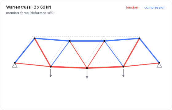
Truss bridge · truss2d
This is a 15-member Warren truss. It is pinned at one end and on a roller at the
other end. There is a 60 kN load at each interior bottom node. The engine
returns the axial force in each member. The bottom chord is in tension. The top chord
is in compression. The mid-span deflection is 9.58 mm.
{
  "title": "Warren truss, 3 x 60 kN",
  "nodes": [[0,0],[4,0],[8,0],[12,0],[16,0],
            [2,3],[6,3],[10,3],[14,3]],
  "materials": { "steel": { "E": 210e9, "nu": 0.3 } },
  "elements": [
    { "type":"truss2d", "nodes":[0,1], "material":"steel", "section":{"A":2e-3} },
    // …bottom & top chords, diagonals (15 members total)
  ],
  "supports": [ {"node":0,"dofs":["ux","uy"]}, {"node":4,"dofs":["uy"]} ],
  "loads": [ {"node":1,"fy":-60000}, {"node":2,"fy":-60000},
             {"node":3,"fy":-60000} ]
}
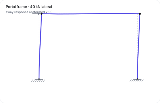
Portal frame · beam2d
This frame has two columns fixed at the base and a beam across the top. There is
a 40 kN lateral (wind) load at the top-left corner. The frame moves sideways by
2.74 mm. The base gets a
48.4 kN·m moment. The system divides each member into parts. Thus the
bending shape is clear.
{
  "title": "Portal frame, 40 kN lateral",
  "nodes": [[0,0],[0,4],[6,4],[6,0]],
  "materials": { "steel": { "E": 210e9, "nu": 0.3 } },
  "elements": [
    { "type":"beam2d", "nodes":[0,1], "material":"steel", "section":{"A":0.012,"I":3e-4} },
    { "type":"beam2d", "nodes":[1,2], "material":"steel", "section":{"A":0.012,"I":3e-4} },
    { "type":"beam2d", "nodes":[2,3], "material":"steel", "section":{"A":0.012,"I":3e-4} }
  ],
  "supports": [ {"node":0,"dofs":["ux","uy","rz"]}, {"node":3,"dofs":["ux","uy","rz"]} ],
  "loads": [ {"node":1,"fx":40000} ]
}
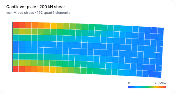
Cantilever plate · quad4
This is a 6 × 2 m plate with a mesh of 192 quad elements. It is clamped
along the left edge. There is a 200 kN downward shear on the right edge. The
engine returns the von Mises stress for each element. The peak is
76.3 MPa in the clamped corners. The tip deflection
is 5.79 mm.
nx, ny, Lx, Ly = 24, 8, 6.0, 2.0
nid = lambda ix, iy: iy*(nx+1) + ix
problem = {
  "materials": {"steel": {"E": 200e9, "nu": 0.3}},
  "nodes": [[x, y] for y in linspace(0,Ly,ny+1)
                    for x in linspace(0,Lx,nx+1)],
  "elements": [
    {"type":"quad4",
     "nodes":[nid(ix,iy),nid(ix+1,iy),nid(ix+1,iy+1),nid(ix,iy+1)],
     "material":"steel", "section":{"t":0.02,"kind":"plane_stress"}}
    for iy in range(ny) for ix in range(nx)
  ],
  "supports": [{"node":nid(0,iy),"dofs":["ux","uy"]} for iy in range(ny+1)],
  "loads": [{"node":nid(nx,iy),"fy":-200000/(ny+1)} for iy in range(ny+1)]
}
Design loop — an agent sizing a beam
This pattern makes physicsbase more than a calculator. Solve the problem. Read the result. Change the design. Solve it again. Repeat until you reach a target factor of safety.
import httpx
YIELD, TARGET = 250e6, 2.0          # Pa, desired factor of safety
I = 4e-6
for _ in range(12):
    problem = build_cantilever(I=I)         # agent's own translation step
    out = httpx.post(API, json=problem).json()
    M = max(abs(e["moment_i"]) for e in out["elements"])
    sigma = M * c / I
    fos = YIELD / sigma
    if fos >= TARGET:
        break
    I *= fos / TARGET * 1.1                 # grow the section, try again
print(f"sized: I={I:.2e} m^4, FoS={fos:.2f}")I; physicsbase is telling it the truth about the
resulting moment and stress.3D building frame · frame3d
This is a single-storey space frame. It has four columns fixed at the base, four roof
beams, and a lateral wind load at a corner. frame3d carries the
axial force, the torsion, and the bending about both local axes at the same time. The roof
diaphragm turns and also moves sideways. Each member returns the
axial_force, the torsion, and the biaxial end moments.
{
  "title": "3D frame, 30 kN corner wind load",
  "nodes": [[0,0,0],[6,0,0],[6,0,5],[0,0,5],
            [0,4,0],[6,4,0],[6,4,5],[0,4,5]],
  "materials": { "steel": { "E": 210e9, "nu": 0.3 } },
  "elements": [
    // 4 columns (0-4,1-5,2-6,3-7) + 4 roof beams (4-5,5-6,6-7,7-4)
    { "type":"frame3d", "nodes":[0,4], "material":"steel",
      "section":{"A":8e-3,"Iy":4e-5,"Iz":4e-5,"J":6e-5} }
    // …7 more members, same section
  ],
  "supports": [
    {"node":0,"dofs":["ux","uy","uz","rx","ry","rz"]},
    {"node":1,"dofs":["ux","uy","uz","rx","ry","rz"]},
    {"node":2,"dofs":["ux","uy","uz","rx","ry","rz"]},
    {"node":3,"dofs":["ux","uy","uz","rx","ry","rz"]}
  ],
  "loads": [ {"node":7,"fx":30000} ]
}
Distributed load + self-weight · element_loads · gravity
This is a cantilever with a uniform line load and its own weight. The system changes distributed
loads into exact equivalent nodal forces and moments. Gravity changes
rho into a body force. With the UDL alone the tip drops
w L⁴ / 8EI = 24.1 mm. The engine gives the same value.
{
  "title": "Cantilever, 4 kN/m UDL + self-weight",
  "nodes": [[0,0],[1,0],[2,0],[3,0]],
  "materials": { "steel": { "E": 210e9, "nu": 0.3, "rho": 7850 } },
  "elements": [
    { "type":"beam2d", "nodes":[0,1], "material":"steel", "section":{"A":0.01,"I":8e-6} },
    { "type":"beam2d", "nodes":[1,2], "material":"steel", "section":{"A":0.01,"I":8e-6} },
    { "type":"beam2d", "nodes":[2,3], "material":"steel", "section":{"A":0.01,"I":8e-6} }
  ],
  "element_loads": [
    {"element":0,"w":[0,-4000]}, {"element":1,"w":[0,-4000]},
    {"element":2,"w":[0,-4000]}
  ],
  "gravity": [0, -9.81],
  "supports": [ {"node":0,"dofs":["ux","uy","rz"]} ]
}
Euler column buckling · analysis: buckling
This is a 3 m pin-ended steel column under axial compression. The buckling
analysis returns the load factor on the applied reference load. For this
section the engine reports a critical load of
≈ 1.84 MN. This is within 1% of the Euler value
Pcr = π²EI/L².
{
  "title": "Pin-ended column buckling",
  "analysis": "buckling", "num_modes": 3,
  "nodes": [[0,0],[0.375,0],[0.75,0], /* …down to */ [3,0]],
  "materials": { "steel": { "E": 210e9, "nu": 0.3 } },
  "elements": [ /* chain of beam2d, section {A:0.02, I:8e-6} */ ],
  "supports": [ {"node":0,"dofs":["ux","uy"]},
                 {"node":8,"dofs":["uy"]} ],
  "loads": [ {"node":8,"fx":-1000} ]   // reference compression
}
// -> { "load_factors": [1842.x, …], "critical_loads": [1.842e6, …] }
Beam natural frequencies · analysis: modal
This is the same cantilever. Here it asks for the vibration modes, not a
deflection. With rho, the engine returns the natural
frequencies. The first frequency is
f₁ = (1.875² / 2π)·√(EI / ρA L⁴) ≈ 9.1 Hz. The engine agrees to
better than 1%.
curl -X POST https://www.physicsbase.dev/modal \
  -d '{ "analysis":"modal", "num_modes":3,
        "nodes": [[0,0], … ,[3,0]],
        "materials": {"steel":{"E":210e9,"nu":0.3,"rho":7850}},
        "elements": [ /* beam2d chain, {A:0.01,I:8e-6} */ ],
        "supports": [{"node":0,"dofs":["ux","uy","rz"]}] }'
# -> { "frequencies_hz": [9.1, 57.0, 159.6], … }
Continuous beam — statically indeterminate · beam2d
This is a two-span beam on three supports under a uniform load. It is statically indeterminate. Thus statics alone cannot find the interior reaction. The engine solves it directly. There is a hogging (negative) moment over the middle support. The interior reaction is larger than the end reactions.
{
  "title": "Two-span continuous beam, 5 kN/m",
  "nodes": [[0,0],[1,0],[2,0],[3,0],[4,0],
            [5,0],[6,0],[7,0],[8,0]],
  "materials": { "steel": { "E": 210e9, "nu": 0.3 } },
  "elements": [ /* 8 beam2d spans, section {A:0.01, I:2e-5} */ ],
  "element_loads": [ /* {element:i, w:[0,-5000]} for i in 0..7 */ ],
  "supports": [ {"node":0,"dofs":["ux","uy"]},
                 {"node":4,"dofs":["uy"]},
                 {"node":8,"dofs":["uy"]} ]
}
// reactions[4].fy is the large interior reaction; the span-0 element
// moment_j over the middle support is negative (hogging).
Multi-storey frame under wind · beam2d
This is a two-storey, one-bay moment frame with lateral loads at each floor. The fixed
column bases carry the overturning. The engine returns the storey drift
(the relative ux between floors) and the column base moments for
design.
{
  "title": "2-storey moment frame, wind",
  // columns at x=0 and x=6; floors at y=0,3,6
  "nodes": [[0,0],[0,3],[0,6],[6,0],[6,3],[6,6]],
  "materials": { "steel": { "E": 210e9, "nu": 0.3 } },
  "elements": [
    {"type":"beam2d","nodes":[0,1],"material":"steel","section":{"A":0.012,"I":3e-4}},
    {"type":"beam2d","nodes":[1,2],"material":"steel","section":{"A":0.012,"I":3e-4}},
    {"type":"beam2d","nodes":[3,4],"material":"steel","section":{"A":0.012,"I":3e-4}},
    {"type":"beam2d","nodes":[4,5],"material":"steel","section":{"A":0.012,"I":3e-4}},
    {"type":"beam2d","nodes":[1,4],"material":"steel","section":{"A":0.012,"I":3e-4}},
    {"type":"beam2d","nodes":[2,5],"material":"steel","section":{"A":0.012,"I":3e-4}}
  ],
  "supports": [ {"node":0,"dofs":["ux","uy","rz"]},
                 {"node":3,"dofs":["ux","uy","rz"]} ],
  "loads": [ {"node":1,"fx":20000}, {"node":2,"fx":20000} ]
}
3D truss tower · truss3d
This is a single bay of a lattice tower. It has a square base and a square top with four legs and cross bracing. There is a vertical load and a lateral load at the top. All members carry axial force only. The engine returns each member force and the 3D displacement of the top node.
{
  "title": "Lattice tower bay",
  // base square z=0 (nodes 0-3), top square z=4 (nodes 4-7)
  "nodes": [[0,0,0],[2,0,0],[2,2,0],[0,2,0],
            [0,0,4],[2,0,4],[2,2,4],[0,2,4]],
  "materials": { "steel": { "E": 210e9, "nu": 0.3 } },
  "elements": [ /* 4 legs (0-4,1-5,2-6,3-7), top ring, base ring, diagonals;
                    every one: type truss3d, section {A:1e-3} */ ],
  "supports": [ /* pin all four base nodes: dofs ["ux","uy","uz"] */ ],
  "loads": [ {"node":4,"fz":-50000,"fx":15000} ]
}
Beam on an elastic foundation · springs
This is a grade beam that rests on soil. A grounded vertical spring at each node models the subgrade (a Winkler foundation). The load pushes the beam into the soil, not into rigid supports. The springs carry the reactions.
k_soil = 2.0e6            # N/m per node (subgrade modulus × tributary length)
problem = {
  "nodes": [[x, 0] for x in range(11)],        # 10 m beam, 1 m spacing
  "materials": {"c": {"E": 30e9, "nu": 0.2}},
  "elements": [ {"type":"beam2d","nodes":[i,i+1],"material":"c",
                 "section":{"A":0.09,"I":6.75e-4}} for i in range(10) ],
  "springs": [ {"node":i,"dof":"uy","k":k_soil} for i in range(11) ],
  # one horizontal restraint stops rigid sliding
  "supports": [ {"node":0,"dofs":["ux"]} ],
  "loads": [ {"node":5,"fy":-120000} ]   # central column load
}
Support settlement · prescribed displacement
Apply a known displacement, not a load. Give a support a
values array. Here the middle support of a continuous beam
moves down 10 mm. The engine returns the extra moments and reactions from
this movement.
"supports": [
  { "node": 0, "dofs": ["ux","uy"] },
  { "node": 4, "dofs": ["uy"], "values": [-0.010] },  // 10 mm settlement
  { "node": 8, "dofs": ["uy"] }
]
Thermal stress in a restrained bar · thermal
Give the material an expansion coefficient alpha. Give each
element a temperature rise dT. A bar is fixed at both ends and
heated. It cannot expand. Thus it gets a compressive stress
σ = −E·α·ΔT. The engine returns this directly.
{
  "title": "Restrained bar, +50°C",
  "nodes": [[0,0],[1,0]],
  "materials": { "steel": { "E": 200e9, "nu": 0.3, "alpha": 12e-6 } },
  "elements": [ {"type":"truss2d","nodes":[0,1],"material":"steel","section":{"A":0.01}} ],
  "supports": [ {"node":0,"dofs":["ux","uy"]}, {"node":1,"dofs":["ux","uy"]} ],
  "thermal": [ {"element":0,"dT":50} ]
}
// elements[0].axial_stress = -E*alpha*dT = -120 MPa (compression)
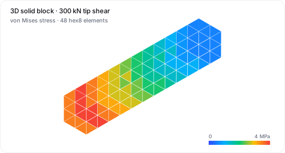
3D solid stress block · hex8 / tet4
This gives full 3D stress with trilinear bricks or linear tets. A clamped block under
end shear returns the 3D stress tensor and the von Mises stress for each element.
The peak (red) is at the fixed face. Build a structured grid of hex8
cells. Clamp one face.
{
  "nodes": [[0,0,0],[1,0,0],[1,1,0],[0,1,0],
            [0,0,1],[1,0,1],[1,1,1],[0,1,1]],
  "materials": { "steel": { "E": 200e9, "nu": 0.3 } },
  "elements": [ {"type":"hex8","nodes":[0,1,2,3,4,5,6,7],"material":"steel"} ],
  "supports": [ /* clamp the x=0 face: nodes 0,3,4,7 in ux,uy,uz */ ],
  "loads": [ /* tension on the x=1 face nodes 1,2,5,6 */ ]
}
// elements[0].stress = [sxx, syy, szz, sxy, syz, szx],  elements[0].von_mises
Axisymmetric pressure vessel · axiquad4
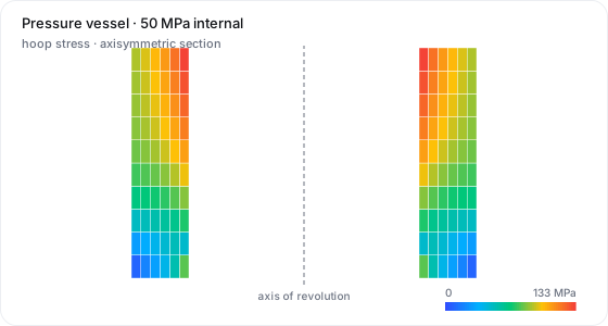
Model a body of revolution in the r-z half-plane. axiquad4
carries the hoop strain automatically. It integrates over the full ring.
Thus nodal loads are total ring forces. Use it for thick cylinders, discs, and
nozzles.
{
  // nodes are [r, z]; keep r > 0 (off the axis)
  "nodes": [[1.0,0],[1.2,0],[1.2,1],[1.0,1]],
  "materials": { "steel": { "E": 200e9, "nu": 0.3 } },
  "elements": [ {"type":"axiquad4","nodes":[0,1,2,3],"material":"steel"} ],
  "supports": [ /* restrain uz on z=0 edge; radial free */ ],
  "loads": [ /* internal pressure as radial ring loads on inner nodes */ ]
}
// stress = [srr, szz, s_hoop, srz] per element
Transient step response · analysis: transient
This is Newmark time integration of the dynamic response. A load comes on suddenly
(a step) and stays. An undamped structure then moves to about twice its
static deflection. This is the dynamic amplification. Add Rayleigh
damping to make it decay.
curl -X POST https://www.physicsbase.dev/transient \
  -d '{ "analysis":"transient", "dt":2e-4, "n_steps":150,
        "damping":[0.5, 1e-5], "monitor":[1,"uy"],
        "nodes": [[0,0], … ], "materials": {"s":{"E":210e9,"nu":0.3,"rho":7850}},
        "elements": [ /* beam2d chain */ ],
        "supports": [{"node":0,"dofs":["ux","uy","rz"]}],
        "loads": [{"node":1,"fy":-5000}] }'
# -> { "peak_displacement": …, "peak_time": …,
#      "monitor": { "history": [ … ] }, "frames": [ … ] }
Combined load + thermal · superposition
Mechanical and thermal effects add in one linear solve. You do not run the cases separately. Here a beam carries a tip load and is heated. The reactions show both at the same time.
{
  "title": "Fixed-fixed beam: load + heating",
  "nodes": [[0,0],[1,0],[2,0],[3,0],[4,0]],
  "materials": { "steel": { "E": 210e9, "nu": 0.3, "alpha": 12e-6 } },
  "elements": [ /* 4 beam2d spans, section {A:0.01, I:8e-6} */ ],
  "supports": [ {"node":0,"dofs":["ux","uy","rz"]},
                 {"node":4,"dofs":["ux","uy","rz"]} ],
  "loads": [ {"node":2,"fy":-8000} ],
  "thermal": [ /* {element:i, dT:40} for each span -> axial thrust */ ]
}
// reactions carry both the bending from the load and the axial
// thrust from restrained thermal expansion, in one solve.
Mixed elements — braced frame · beam2d + truss2d
Different element types share one model. Use rigid beam2d members
for the moment frame. Use pin-ended truss2d diagonals for the
bracing. The engine assembles them into one stiffness matrix. The braces
carry axial force. The frame carries bending.
  "elements": [
    {"type":"beam2d","nodes":[0,1],"material":"s","section":{"A":0.012,"I":3e-4}},
    {"type":"beam2d","nodes":[1,2],"material":"s","section":{"A":0.012,"I":3e-4}},
    {"type":"beam2d","nodes":[3,2],"material":"s","section":{"A":0.012,"I":3e-4}},
    {"type":"truss2d","nodes":[0,2],"material":"s","section":{"A":6e-4}},  // diagonal brace
    {"type":"truss2d","nodes":[3,1],"material":"s","section":{"A":6e-4}}   // diagonal brace
]beam2d (which adds rz) and truss2d
mix freely in 2D. The truss does not use the rotational DOF.
physicsbase now has these functions. There are shell elements (shell4). There is geometric nonlinearity (large-displacement and snap-through). There is material nonlinearity (J2 plasticity and continuum damage). There is contact (rigid barriers, deformable node pairs, and node-to-surface on non-matching meshes). There is finite-strain hyperelasticity (compressible Neo-Hookean, with full Newton-Raphson on continuum elements). There is steady-state harmonic dynamics (damped frequency response). There is Coulomb frictional contact (stick and slip). There is a multi-step load-stepping framework (*STEP-style). There is a full composites stack: orthotropic lamina, laminate ABD (CLT), fibre and matrix homogenization, Hashin progressive ply-failure, oxidation reaction-diffusion, and a pluggable UMAT user-material hook. Since then it has also added large-strain and rate-dependent materials (finite-strain J2 plasticity, Perzyna viscoplasticity, Prony viscoelasticity, Norton creep, Lemaitre damage-plasticity), fatigue (stress-life, Paris crack growth, strain-life), viscous CFD (Stokes, steady and transient Navier-Stokes), acoustics (cavity modes, driven response) and multiphysics coupling (two-way thermo-mechanical, piezoelectric, vibro-acoustic, 2D magnetostatics). We numerically verify each one against a recorded reference; this is not experimental validation. The remaining frontier is large-sliding and self-contact, turbulence and fluid-structure interaction, explicit/dynamic contact, and time-harmonic electromagnetics.