How the structure designs itself.
We reproduced the classic topology-optimization method on the physicsbase engine. This is the method behind the organic, bone-like optimal structures. The FE solve is ours. The loop around it is the algorithm. It produced the well-known optimized cantilever.
Give a mechanical engineer a rectangle of steel, a place to bolt it down, and a load to carry. In time they ask the question that started a whole field: where should the material go? Not "is this beam strong enough," but "of all the ways to spend this much metal, which layout is stiffest?" That question is topology optimization. Its answers look like nature: branching struts, arches, and trusses that no one drew by hand.
The main method is SIMP (Solid Isotropic Material with Penalization). It is a finite-element solve, run again and again inside an optimization loop. This makes it a good test for physicsbase. The whole idea of physicsbase is to be the FE kernel that an agent calls many times. So we built SIMP on top of the engine. We ran it on two textbook problems. Here is how it works, what came out, and why the solve-in-a-loop shape is important.
The problem, precisely
Take a design domain. Divide it into finite elements. Give each element e a density variable \(\rho_e\) between 0 (void) and 1 (solid). The stiffness of that element scales with its density through a penalized power law:
The exponent is the key. With p = 3, a half-dense element gets only ⅛ of the stiffness for half the material. Thus intermediate "grey" densities are inefficient, and the optimizer moves toward clear black-and-white designs. We then minimise compliance (the strain energy of the structure, \(c = \mathbf{F}^{\mathsf T}\mathbf{u}\); low compliance means high stiffness). We do this with a fixed material budget, for example 40% of the domain.
At the boundary: what actually crosses the wire
Here is the whole relationship in one exchange. In each iteration, the agent gives physicsbase a description of the current design as one JSON object. This is the geometry, the material of each element, where it is held, and the loads. Nothing else. This is a real request to the engine (reduced to a two-element patch so it fits on the page):
"nodes": [[0,0],[1,0],[2,0],[0,1],[1,1],[2,1]],
"materials": { "steel": { "E": 200e9, "nu": 0.3 } },
"elements": [
  { "type":"quad4", "nodes":[0,1,4,3], "material":"steel", "section":{"t":0.01}, "id":"e0" },
  { "type":"quad4", "nodes":[1,2,5,4], "material":"steel", "section":{"t":0.01}, "id":"e1" }
],
"supports": [ {"node":0,"dofs":["ux","uy"]}, {"node":3,"dofs":["ux","uy"]} ],
"loads": [ {"node":2,"fy":-5000}, {"node":5,"fy":-5000} ]
physicsbase solves it and returns the answer: the deformation at each node, the reactions at the supports, and the stress in each element. The optimizer reads these numbers. This is the real response (rounded):
"displacements": [
  { "ux": 0.0,        "uy": 0.0 },          // node 0 — held
  { "ux": -3.03e-5,   "uy": -4.33e-5 },
  { "ux": -4.04e-5,   "uy": -1.271e-4 },     // node 2 — loaded corner
  /* … nodes 3–5 … */
],
"reactions": [ { "fx": 625.0, "fy": 5000.0 }, /* … */ ],  // supports carry the 10 kN
"elements": [
  { "id": "e0", "stress": [0, 0, -1.00e6], "von_mises": 1.73e6 },
  { "id": "e1", "stress": [0, 0, -1.00e6], "von_mises": 1.73e6 }
],
"summary": { "n_dof": 12, "max_abs_displacement": 1.27e-4, "solve_ms": 0.9 }
Turning the response back into the next request
This is where the loop is. From the response, the optimizer computes the strain energy of each element, which shows how hard that element works. It uses the returned displacements. Elements that store a lot of energy are load paths to reinforce. Elements that are idle are material to spend elsewhere. So the agent rewrites the design and sends it back:
# each element's material stiffness now reflects its density:
#   busy elements  -> denser (stiffer material) in the next request
#   idle elements  -> lighter (softer material) in the next request
response  = physicsbase.solve(design)        # ← displacements, stresses
energy    = strain_energy_from(response)      # read the numbers
design    = redistribute(design, energy)      # → new material per element
# ...repeat ~50 times. every step stands on one real solve.
After fifty requests, the material has moved to where the responses said it was needed. Then the shapes below appear.
Under the hood: physicsbase as the finite-element kernel
Each of those requests is a linear FE solve of \(\mathbf{K}(\rho)\,\mathbf{u} = \mathbf{F}\). The global stiffness comes from element stiffnesses, scaled by the current density of each element. This is what physicsbase does inside. Its plane-stress quad4 element and assembly are numerically verified against analytical solutions. For the tight 50-solve loop in the reference script, we call the element formulation directly, to skip the JSON round-trip for speed. But the object that crosses the boundary is the same one shown above:
# the FE kernel comes from physicsbase — a numerically verified element
from femengine.elements import Quad4
from femengine.materials import Material

# 8x8 unit-square plane-stress stiffness, E = 1
KE = Quad4.stiffness([[0,0],[1,0],[1,1],[0,1]],
                     Material(E=1.0, nu=0.3), {"t":1.0, "kind":"plane_stress"})

for it in range(max_iter):
    E   = Emin + x**penal * (E0 - Emin)          # SIMP interpolation
    K   = assemble(KE, E, edof)                    # scale & scatter each element
    U   = solve(K, F, free)                       # the physicsbase FE solve
    ce  = einsum('ej,jk,ek->e', Ue, KE, Ue)      # element strain energy
    dc  = -penal * x**(penal-1) * (E0-Emin) * ce  # compliance sensitivity
    dc  = filter(dc)                             # density filter (kills checkerboards)
    x   = oc_update(x, dc, volfrac)              # optimality-criteria step
Three parts make it converge, rather than become a pixelated checkerboard. They are all standard. First, the compliance sensitivity \(\frac{\partial c}{\partial \rho_e} = -p\,\rho_e^{\,p-1}(E_0 - E_{\min})\,\mathbf{u}_e^{\mathsf T}\mathbf{k}_0\mathbf{u}_e\), which is the contribution of each element to the stiffness change. Second, a density filter, which blurs the sensitivities over a small radius to set a minimum feature size. Third, the Optimality-Criteria update, a simple fixed-point rule that moves material to where it helps most, while a bisection holds the volume constraint.
The one call that is the physics
It is worth being clear about how little of this is physicsbase and how much of it is. The whole contribution of the engine is one function call:
>>> KE = Quad4.stiffness([[0,0],[1,0],[1,1],[0,1]],
...                     Material(E=1.0, nu=0.3),
...                     {"t": 1.0, "kind": "plane_stress"})
>>> KE.shape
(8, 8)          # 4 corners × 2 DOFs (ux, uy) = 8
That 8×8 matrix is the plane-stress stiffness of one element. It is the same numerically verified quad4 that passes the uniform-strain patch test in the engine's own suite. Two settings matter for real work. section["kind"] chooses plane_stress (a thin sheet, with zero out-of-plane stress) or plane_strain (a thick body, with zero out-of-plane strain). section["t"] is the thickness. We evaluate it one time, on a unit square with E = 1, because on a regular grid every element has the same geometry. Thus a scale of that single matrix by the SIMP modulus of each element is the assembly. There is no other physics in the program.
Turning a response into a sensitivity
The optimizer asks one thing of every solve: the strain energy in each element, \(\mathbf{u}_e^{\mathsf T}\mathbf{k}_0\mathbf{u}_e\). Everything to compute it is in the response. Take the eight displacement components of each element from the returned displacements. Then contract them with the same KE that physicsbase gave you:
# response["displacements"] -> a flat DOF vector U
U  = np.array([[d["ux"], d["uy"]] for d in resp["displacements"]]).ravel()
Ue = U[edof]                              # (n_elem, 8): each element's DOFs
ce = np.einsum('ej,jk,ek->e', Ue, KE, Ue)   # strain energy per element

# physicsbase also hands back per-element stress & strain directly,
# so the same quantity is available as an energy density with no re-derivation:
#   resp["elements"][e]["stress"], resp["elements"][e]["strain"]
This is the key point of the usage story: physicsbase returns fields that the agent can act on. The displacements array is indexed by node. The elements array carries stress, strain, and von_mises for each element, keyed by the id that you sent in. You derive nothing again. The sensitivity is a dot product over numbers that the engine already computed.
In-process or over the wire — the same object
There are two ways to reach that solve. They return the same numbers. For the tight fifty-iteration loop, the reference script imports Quad4 and assembles in the same process, with no serialization. This is the fastest way. An agent that runs from elsewhere sends the JSON problem shown earlier to /solve with POST. It reads the same displacements and elements back. The physics, the element, and the returned fields are the same. You choose the transport that fits where your loop runs.
What came out
We ran two standard benchmarks. First, a cantilever: clamp the left edge, put a load at the middle of the right edge, and spend 40% of the box. We gave the optimizer a uniform grey slab. It ran for 50 iterations (about 15 seconds).

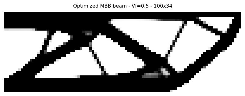
That shape is not designed. It is discovered. The optimizer rebuilt the load path that an engineer would draw, from "minimise compliance" alone. There is a top chord and a bottom chord in tension and compression. Diagonals carry the shear. Closed triangular cells give stiffness. Run the classic MBB beam instead (a simply-supported span pushed down at the top centre). Then you get the other known result:
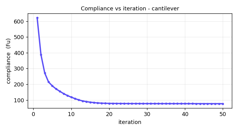
The optimization behaves well. The compliance falls fast for the first twelve iterations. Then it flattens as the topology sets. The design has found its structure. After that it only refines the edges.
Why the loop is the point
Topology optimization is the clearest example of the pattern that physicsbase exists for. No one solves this one time. It is solve → read the strain energy → redistribute material → solve again, fifty times. Each step depends on the real numbers from the last step. Give an agent an FE library, and it must derive the assembly, the boundary conditions, and the sensitivities again each time. It will get one of them subtly wrong. Give it an FE solve as an API call, and the loop is easy to drive. The agent owns the design logic. The engine owns the physics. Every iteration stands on a numerically checked solve.
This is the same argument as sizing a beam or checking a factor of safety. It just has fifty times more solves and a much better-looking answer.
The complete code
Here is the whole optimizer, exactly as it ran to produce the figures above.
It is one file. It stands on physicsbase's Quad4 for the physics. There are no
hidden helpers.
"""SIMP compliance topology optimization, built on the physicsbase engine.

physicsbase supplies the finite-element kernel: the 8x8 plane-stress Quad4
element stiffness is taken straight from femengine.elements.Quad4 — the same
numerically verified element used elsewhere in the engine. Everything else (the SIMP
interpolation, compliance sensitivities, density filter, and the
Optimality-Criteria update) is the optimization loop wrapped around it.
"""
import sys
from pathlib import Path

import numpy as np
from scipy.sparse import coo_matrix
from scipy.sparse.linalg import spsolve

sys.path.insert(0, str(Path(__file__).resolve().parents[1]))
from femengine.elements import Quad4               # physicsbase FE kernel
from femengine.materials import Material


def unit_element_stiffness(nu=0.3):
    """8x8 plane-stress stiffness of a unit square Quad4 with E = 1."""
    coords = [[0, 0], [1, 0], [1, 1], [0, 1]]        # CCW
    return Quad4.stiffness(coords, Material(E=1.0, nu=nu),
                           {"t": 1.0, "kind": "plane_stress"})


def build_filter(nelx, nely, rmin):
    """Linear (cone) density filter weights as a sparse operator."""
    nel = nelx * nely
    rows, cols, vals = [], [], []
    R = int(np.ceil(rmin)) - 1
    for i in range(nelx):
        for j in range(nely):
            e = i * nely + j
            for ii in range(max(i - R, 0), min(i + R + 1, nelx)):
                for jj in range(max(j - R, 0), min(j + R + 1, nely)):
                    w = rmin - np.hypot(i - ii, j - jj)
                    if w > 0:
                        rows.append(e); cols.append(ii * nely + jj); vals.append(w)
    H = coo_matrix((vals, (rows, cols)), shape=(nel, nel)).tocsr()
    Hs = np.asarray(H.sum(axis=1)).ravel()
    return H, Hs


def optimize(nelx=120, nely=60, volfrac=0.4, penal=3.0, rmin=2.4,
             load="cantilever", max_iter=90, move=0.2, tol=0.01):
    ndof = 2 * (nelx + 1) * (nely + 1)
    KE = unit_element_stiffness()

    # element -> global DOF map (node i,j -> id i*(nely+1)+j)
    edof = np.zeros((nelx * nely, 8), dtype=int)
    for i in range(nelx):
        for j in range(nely):
            n1 = i * (nely + 1) + j              # bottom-left
            n2 = (i + 1) * (nely + 1) + j        # bottom-right
            n3 = (i + 1) * (nely + 1) + j + 1    # top-right
            n4 = i * (nely + 1) + j + 1          # top-left
            edof[i * nely + j] = [2*n1, 2*n1+1, 2*n2, 2*n2+1,
                                  2*n3, 2*n3+1, 2*n4, 2*n4+1]
    iK = np.kron(edof, np.ones((8, 1), int)).flatten()
    jK = np.kron(edof, np.ones((1, 8), int)).flatten()

    # boundary conditions and unit load
    F = np.zeros(ndof); fixed = []
    if load == "cantilever":                     # clamp left edge, load right-mid
        for j in range(nely + 1):
            fixed += [2*j, 2*j+1]
        ntip = nelx * (nely + 1) + (nely // 2)
        F[2*ntip + 1] = -1.0
    else:                                        # MBB half-beam
        for j in range(nely + 1):
            fixed.append(2*j)                    # symmetry: left edge ux = 0
        fixed.append(2*(nelx*(nely+1)) + 1)      # bottom-right roller: uy = 0
        F[2*nely + 1] = -1.0                     # load at top-left
    fixed = np.array(sorted(set(fixed)), dtype=int)
    free = np.setdiff1d(np.arange(ndof), fixed)

    H, Hs = build_filter(nelx, nely, rmin)
    x = np.full(nelx * nely, volfrac)

    for it in range(max_iter):
        Emin, E0 = 1e-9, 1.0
        E = Emin + x**penal * (E0 - Emin)                    # SIMP interpolation
        sK = (KE.flatten()[np.newaxis]).T * E
        K = coo_matrix((sK.flatten(order='F'), (iK, jK)),
                       shape=(ndof, ndof)).tocsc()
        K = 0.5 * (K + K.T)
        U = np.zeros(ndof)
        U[free] = spsolve(K[free][:, free], F[free])         # the FE solve

        Ue = U[edof]
        ce = np.einsum('ej,jk,ek->e', Ue, KE, Ue)            # element strain energy
        comp = float(np.sum(E * ce))
        dc = -penal * x**(penal - 1) * (E0 - Emin) * ce      # compliance sensitivity
        dv = np.ones(nelx * nely)

        dc = np.asarray(H @ (dc / Hs))                       # density filter
        dv = np.asarray(H @ (dv / Hs))

        l1, l2 = 0.0, 1e9                                    # OC update (bisection)
        while (l2 - l1) / (l1 + l2 + 1e-30) > 1e-4:
            lm = 0.5 * (l1 + l2)
            xn = np.clip(x * np.sqrt(np.maximum(-dc, 0) / (dv*lm + 1e-30)),
                         np.maximum(0.0, x - move), np.minimum(1.0, x + move))
            xn = np.clip(xn, 0.001, 1.0)
            l1, l2 = (lm, l2) if xn.mean() > volfrac else (l1, lm)
        change = float(np.max(np.abs(xn - x)))
        x = xn
        print(f"it {it:3d}  compliance {comp:10.4f}  vol {x.mean():.3f}")
        if change < tol:
            break
    return x.reshape(nelx, nely).T


if __name__ == "__main__":
    dens = optimize()
    np.save("topopt_density.npy", dens)
    print("final volume fraction:", dens.mean())
That is the whole program. The one import that matters — from femengine.elements import Quad4 — is where physicsbase does the work. The rest is the classic algorithm. Run it, and the structures above appear.
Honest footnotes
What we implemented is the standard density-based method as described across the references below — the mathematics is common to all of them and to any graduate course on the subject. The code is our own, written around physicsbase's element; we did not reuse any of the published implementations. Our version is 2D minimum-compliance with a linear density filter and an OC update; it does not include the parallel solvers, 3D extension, or advanced projection filters that make the cited "large-scale" codes special. The point here was not to beat them — it was to show that a general-purpose FE engine, called in a loop, reproduces the canonical result cleanly. It does.
References
- M. P. Bendsøe & O. Sigmund, Topology Optimization: Theory, Methods, and Applications, Springer (2003) — the standard text for the SIMP method.
- O. Sigmund, "A 99 line topology optimization code written in Matlab," Structural and Multidisciplinary Optimization 21 (2001), 120–127.
- F. Ferrari & O. Sigmund, "A new generation 99 line Matlab code for compliance topology optimization and its extension to 3D," Struct. Multidisc. Optim. (2020). arXiv:2005.05436
- A. Gupta, R. Chowdhury, A. Chakrabarti & T. Rabczuk, "A 55-line code for large-scale parallel topology optimization in 2D and 3D" (2020). arXiv:2012.08208
examples/topopt.py in the engine repo. It is built entirely on physicsbase's quad4. Give it your own domain, loads, and volume budget. Then a structure appears. Read the docs →